7 - Feature Analysis

1.0 Introduction

The tutorial uses the example file Examppit.dips8. The data has been collected by a geologist working on a single rock face above the first bench in a young open pit mine.

The rock face above the current floor of the existing pit has a dip of 45 degrees and a dip direction of 135 degrees. The current plan is to extend the pit down at an overall angle of 45 degrees. This will require a steepening of the local bench slopes, as indicated in the figure above. The local benches are to be separated by an up-dip distance of 16 m. The bench roadways are 4 m wide.

Topics Covered in this Tutorial:

• Add User Plane
• Add Sets from Cluster Analysis
• Symbolic Pole Plot
• Qualitative Chart

Finished Product:

The finished product of this tutorial can be found in the Tutorial 07 Feature Analysis .dips8 files, located in the Examples > Tutorials folder in your Dips installation folder.

2.0 Model

If you have not already done so, run Dips by double-clicking on the Dips icon in your installation folder. Or from the Start menu, select Programs > Rocscience > Dips > Dips.

If the Dips application window is not already maximized, maximize it now, so that the full screen is available for viewing the model.

Dips comes with several example files installed with the program. These example files can be accessed by selecting File > Recent Folders > Examples Folder from the Dips main menu. This tutorial will use the Examppit.dips8 file to demonstrate the basic plotting features of Dips.

1. Select File > Recent Folders > Example Folder from the menu .
2. Open the Examppit.dips8 file. Since we will be using the Examppit.dips8 file in other tutorials, save this example file with a new file name without overwriting the original file.
3. Select File > Save As from the menu.
4. Enter the file name Tutorial 07 Feature Analysis and Save the file.

You should see the Stereonet Plot View shown in the following figure.

If you do not see the plot below, then use the Sidebar Plot Options to view pole vectors and contours on the stereonet.

5. Switch to the Grid Data view of the input data using the tabs at the lower left of the view.

The Examppit.dips8 file contains 303 rows, and the following columns:

• The two mandatory Orientation columns
• A Traverse column
• 5 Extra Columns ( Spacing, Length, Type, Shape, Surface)

Let’s examine the Project Settings information for this file.

2.1 PROJECT SETTINGS

1. Select Project Settings from the toolbar or the Analysis menu.
2. In the Project Settings dialog:
   
   Note the following:
   • The Global Orientation Format = Dip/Dip Direction
   • The Declination = 7.5 degrees, indicating that 7.5 degrees will be added to the dip direction of the data, to correct for magnetic declination
   • The Quantity Column is not used in this file, so each row of the file represents an individual measurement.

2.2 TRAVERSES

Let’s inspect the Traverse Information.

1. Select the Traverses button in the Project Settings dialog (the Traverses dialog is also available directly in the Analysis menu).
   
   As you can see in the Traverse Information dialog, this file uses only a single Traverse:
• The Traverse Type is Planar, with a Dip = 45 degrees and a Dip Direction = 135 degrees (i.e., the face above the survey bench, as you can read in the Comments).
• Note that the Traverse Format is the same as the Global Orientation Format ( Dip / Dip Direction), as we would expect for a file with only a single Traverse defined.
2. Select Cancel in the Traverse Information dialog.
3. Select Cancel in the Project Settings dialog.
4. Switch back to the Stereonet Plot view.

Before we proceed with the Kinematic Analysis, we will:

• Add the slope plane to the view
• Create a Symbolic Plot
• Define sets for the main data clusters
• Estimate the friction angle from the joint surface condition

3.0 Add Plane

Let’s add the slope plane to the stereonet.

1. Select Add User Plane from the toolbar or Planes menu.
2. Click the mouse anywhere in the stereonet.
3. In the Add User Plane dialog:
1. Enter ID = 1.
2. Enter Label = pit slope.
3. Set Convention = Dip / Dip Direction in the dropdown.
4. Enter Orientation coordinates Dip / Dip Direction = 45 / 135.



5. Select OK.

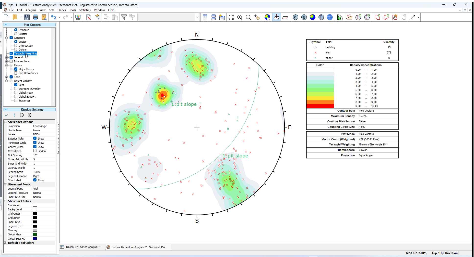
You should see the pit slope plane as shown below.

4.0 Symbolic Pole Plot

Feature attribute analysis can be carried out on a Pole Plot with the Symbolic Plot option. Let’s create a Symbolic Pole Plot based on the discontinuity type (i.e., the data in the TYPE column).

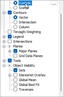
1. In the Sidebar Plot Options, select Pole Vector Display > Symbolic
2. Select the small button which appears at the right.



3. In the Symbolic Plot Options dialog:
4. Set Data Type = TYPE. The data in the TYPE column is Qualitative which is the default selection.
   
5. Select OK to generate the Symbolic Plot.

Look closely at the data clustering and the data TYPE. Most of the features are joints as indicated in the Legend. Note the clustering of bedding features and the two clusters of shear features. These may behave very differently from similarly oriented joints or extension fractures, and should be considered separately.

Although the shear features are not numerous enough to be represented in the contours (the number of mapped shears is small), they may have a dominating influence on stability due to low friction angles and inherent persistence. It is always important to look beyond mere orientations and densities when analyzing structural data.

5.0 Contour Plot

Let’s examine the data contours.

A useful rule of thumb is that any cluster with a maximum concentration of:

• Greater than 6% is very significant.
• 4-6% represents a marginally significant cluster.
• Less than 4% should be regarded with suspicion unless the overall quantity of data is very high (several hundreds of poles).

Rock mechanics texts give more rigorous rules for statistical analysis of data.

Now apply the Terzaghi Weighting to the data, to account for bias correction due to data collection on the (Planar) Traverse.

1. Select the Terzaghi Weighting checkbox in the Sidebar Plot Options .
   

Observe the change in adjusted concentration for the set nearly parallel to the mapping face (the “bedding plane” joint set).

2. Turn off the Terzaghi Weighting checkbox in the Sidebar Plot Options to restore the original unweighted plot.

See the Terzaghi Weighting topic for more information about the Terzaghi Weighting procedure used in Dips.

6.0 Creating Sets

Let’s use the Sets from Cluster Analysis option to delineate the joint contours and create four Sets from the four major data concentrations on the stereonet.

1. Select Sets from Cluster Analysis option from the toolbar or Sets menu.
2. In the Sets from Cluster Analysis dialog:
1. Enter Limit Cluster Size to Cone with Maximum Angle = 25 degrees.
2. Click the Select button.



3. Use the mouse to click on the approximate center of the four main data clusters on the stereonet.
4. Right-click and select Done .

Turn on the display of User Plane and Mean Set Planes:

5. Select Legend > Major Planes checkbox in the Sidebar Plot Options.

You should see the Set Windows shown below.

Turn off the display of the Mean Set Planes and the pit slope:

6. Unselect Planes > Major Planes checkbox in the Sidebar Plot Options.

7.0 Estimating Friction Angle

For stability analysis it will be necessary to assume a value for friction angle on the joint surfaces.

For the purpose of estimating a friction angle, we will create a Chart of the data in the SURFACE column of the Examppit.dips8 file.

1. Select Analysis > Chart from the menu.
2. In the Chart dialog:
1. Select Data = SURFACE from the dropdown.
2. Keep the Data to Plot = Qualitative unchanged.
3. Keep the Plot Type = Column unchanged.
4. Keep the Set Filter = None unchanged. All four Sets will be considered.



5. Select OK.

A Qualitative column chart of SURFACE data is generated.

From the chart, the surfaces are about 50 percent rough (considering both “ rough” and “ v.rough” features) and 50 percent " smooth", so we will assume an average friction angle of 30 degrees for all features.

This concludes the tutorial. You are now ready for the next tutorial, Tutorial 08 - Kinematic Analysis (Flexural Toppling).