6 - Point Cloud Geometry and Barrier Analysis
This tutorial demonstrates the creation and modification of a slope surface from a point cloud. Using the heatmap feature, we'll then determine a barrier placement location, and the required barrier capacity and height. Lastly, the 3D barrier plot feature is demonstrated for the analysis of critical barrier sections in 3D space.
Topics Covered in this Tutorial:
- Surface Triangulation Tools (Add Surface From Points, Simplify)
- Geometry Repair Tools
- Topographic Lines
- Point Seeders
- Surface Heatmap
- Barrier Design
- Barrier Plots in 3D
Finished Product:
The finished product of this tutorial can be found in the Tutorial 06 Point Cloud Geometry and Barrier Analysis data file. All tutorial files installed with RocFall3 can be accessed by selecting File > Recent Folders > Tutorials Folder.
1.0 Import Point Cloud File
Open a new document in RocFall3, if not already done so. Maximize the window so the full-screen space is available for model construction and viewing. In RocFall3, the slope can be created from a point cloud, a surface mesh geometry, lines/contours, extrusion of an existing RocFall2 file, import of RS3/
Slide3 files, or import of a digital elevation model via satellite data (Import Terrain). This tutorial demonstrates the process of importing a slope geometry from a provided point cloud data file.
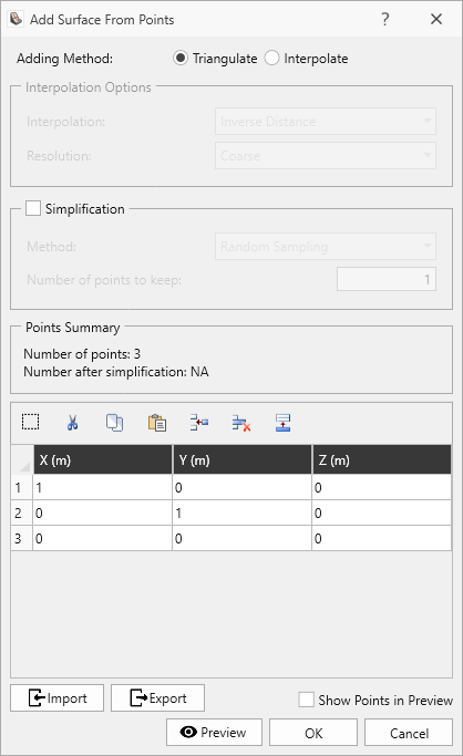
- Select Geometry > Surface Triangulation Tools > Add Surface from Points

-
Select Import
 , located on the bottom-left corner of the dialog.
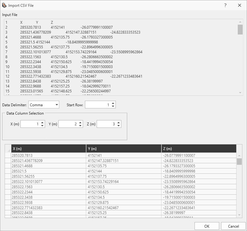
- Open the provided Tutorial 6 Surface Points.txt file in the Tutorials Folder. By default, the installation program puts all supporting files for tutorials in: C:\Users\Public\Documents\Rocscience\RocFall3 Examples\Tutorials
- The Import CSV File dialog displays a preview of the coordinates. The Data Delimiter should be set to Comma with a Start Row of 1.
- In
the Data Column Selection section, enter:
- X = 1
- Y = 2
- Z = 3
Click OK.
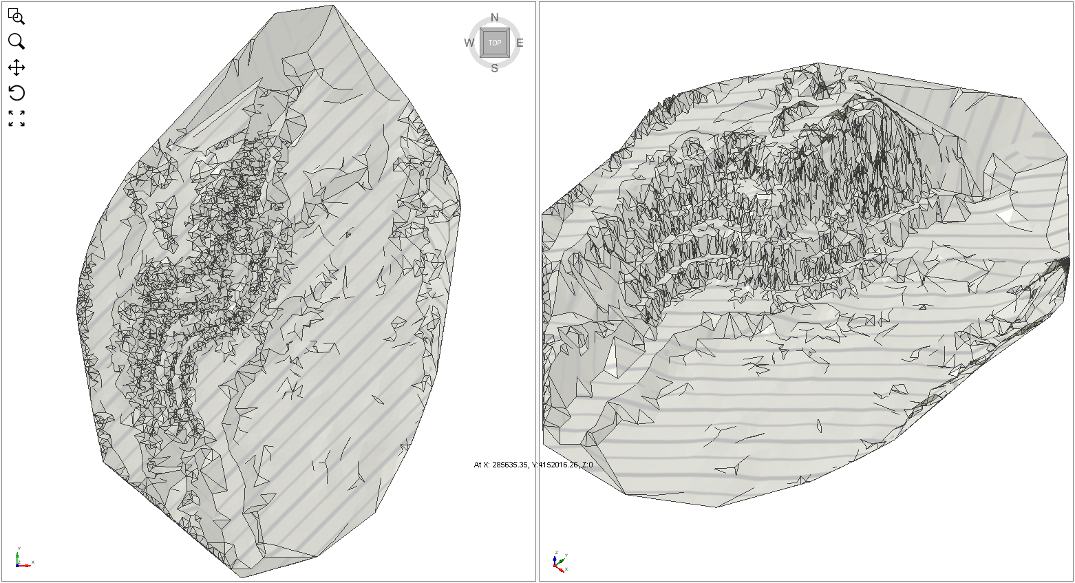
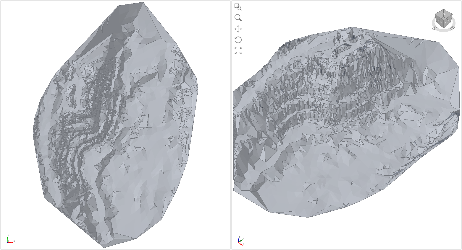
- Back in the Add Surface From Points dialog, 5326 points are displayed. Select Preview to review the surface geometry in the viewports. The dialog can be moved around to view all parts of viewports.
- Click OK to import the point cloud.
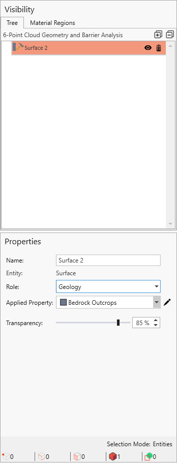
- A "Surface" entity generated from the point cloud data should now be available in the visibility tree. Select the Surface from the Visibility tree and change its Role to Geology in the Properties pane:
2.0 Simplify Triangulation
It is good practice to check the number of surface triangles generated from geometry import and to simplify the surface triangulation as needed. The number of triangles for use should depend on the purpose of the analysis but should always be considered in conjunction with computer specifications for optimal performance.
This section demonstrates the Simplify Triangulation tool for modifying the number of triangles in the slope mesh.
- Select the Surface entity from the Visibility Tree. Then select Geometry > Surface Triangulation Tools > Simplify Triangulation
 in the menu.
 - The Simplify Triangulation dialog shows the current surface triangulation as well as a summary of the number of triangles. Under Simplification Level, select Coarse (5000).
- Select Preview to update the surface in the preview.
- Click OK to accept the new surface triangulation.
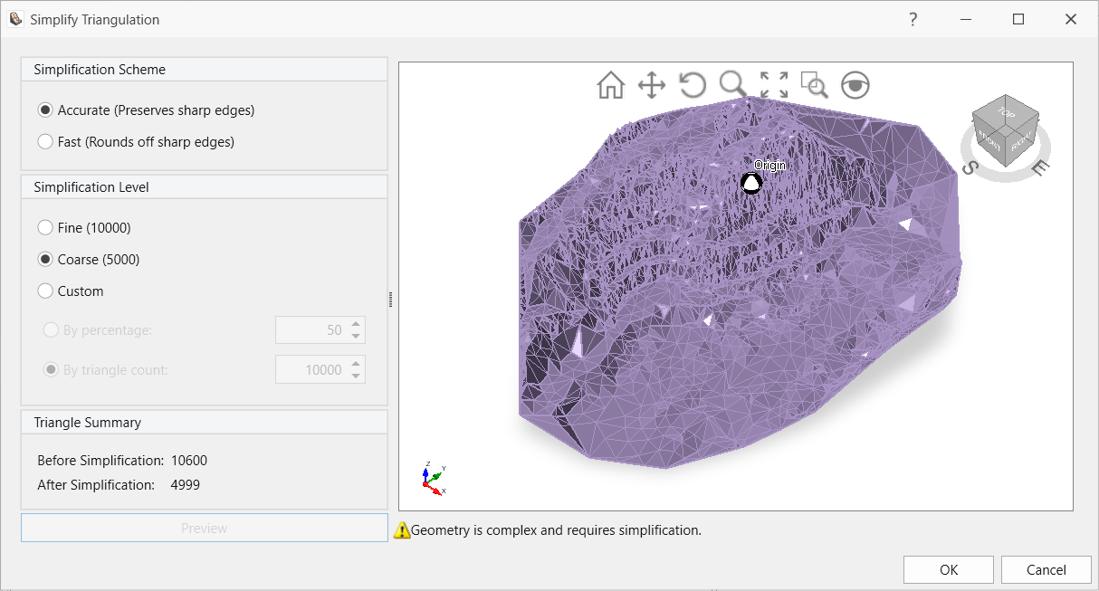
Surface Triangulation Dialog
3.0 Repair Geometry
RocFall3 has a built-in geometry repair tool that can find and repair defects in a geometry entity. This tool is recommended every time after importing or modifying a geometry.
- Select the simplified point cloud surface in the Visibility Tree, and then select Geometry > Repair Geometry
 in the menu.
 - The Repair Geometry dialog shows the total number of defects in the selected geometry and the locations of these defects. Click the Repair button. Repair All first re-triangulates the surface triangles to achieve better aspect ratios and then repairs all defects. Notice how the number of defects has reduced to zero for all except 1 Near-Degenerate triangle. If we select Repair again, this will also be removed.
- Click Close when done repairing.
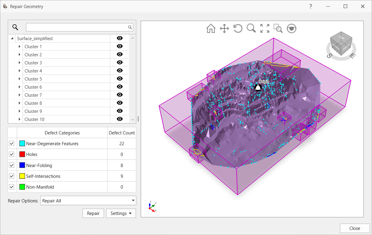
Repair Geometry Dialog
4.0 Set Slope Surface
As the program can accommodate more than one surface geometry, the user would need to establish which surface should be used for calculations using the Set Slope Surface function.
- Select the surface entity from the Visibility Tree and then select Geometry > Set Slope Surface in the menu.
Notice the surface colour has changed. The colour comes from the material property "Bedrock Outcrops", which is the default first material in the material properties list. Set Slope Surface automatically assigns the material "Bedrock Outcrops" to the entire slope surface.
5.0 Material Properties
- Select Materials > Define Materials in the menu, or click the Define Materials
 icon in the toolbar.
The Material Properties dialog shows three pre-defined materials. These can be modified and deleted. New materials can also be added. For this tutorial, the default materials and their properties will be used, so select Cancel.
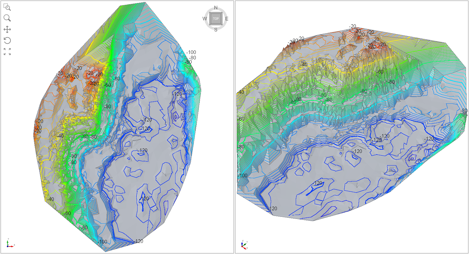
6.0 Topographic Lines
- Select Annotate > Topographic Lines, or click the Topographic Lines
 icon in the toolbar.
Topographic lines help to visualize the topography of the surface model and to provide guidance for the assignment of seeders (rock origins), materials and protection systems. The viewports should now be updated with topographic lines. To change the contour density, select the Topographic Annotation entity in the Visibility Tree and modify its properties from the Properties pane below:
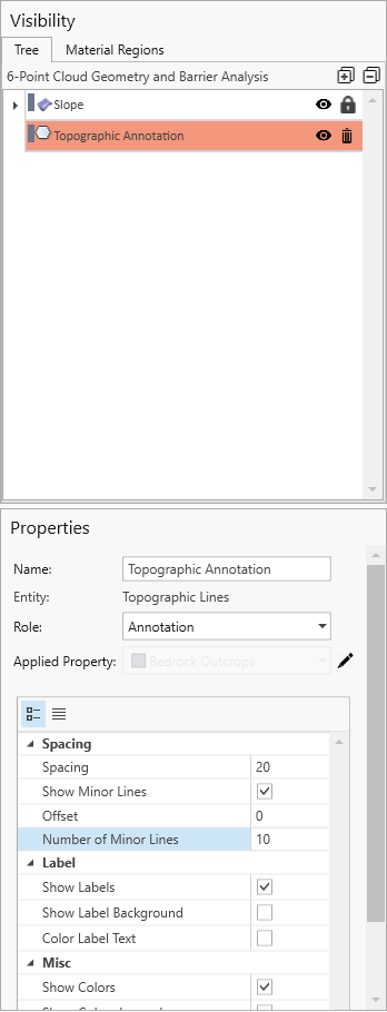
- Enter a Spacing of 20 and Number of Minor Lines of 10. Click anywhere on the viewport to update the topographic lines.
7.0 Add a Point Seeder
Add a point seeder to model a point source of bodies.
- Select Seeder > Add Point Seeder
 . Change the Select Point dropdown to Enter Coordinates and enter the following coordinates: (285376, 4152111, -53).
 - Click OK.
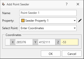
A Point Seeder entity should appear in the Visibility Tree and on the slope.
Alternatively, a point seeder can be placed on the slope by left-clicking in the viewport.
8.0 Define Seeder Properties
For this tutorial, 400 rocks are seeded and assumed to fall due to blasting, which means they may have a non-zero initial velocity.
- Select Seeder > Define Seeder Properties

- For Seeder Property 1, navigate to the Number of Rocks tab and set the value to 400.
- Navigate to the Initial Velocity tab. See the table below for the Mean, Std. Dev, Rel Min, and Rel Max for the translational velocity, Trend, and Plunge. A Normal Distribution is used for all parameters.
| Property | Distribution | Mean | Std. Dev. | Rel. Min. | Rel. Max |
| Translational Velocity | Normal | 1 | 1 | 1 | 1 |
Trend | Normal | 105 | 15 | 45 | 45 |
| Plunge | Normal | 0 | 30 | 90 | 90 |
9.0 Compute
- Select Analysis > Compute in the menu, or click the Compute
 icon in the toolbar.
10.0 Results and Analysis
- After the model has finished computing, navigate to the Results workflow tab to view results.
- Turn off the topographic line visibility to see the trajectories more clearly. Simply select the 'eye icon'
 next to the topographic lines entity in the Visibility Tree.
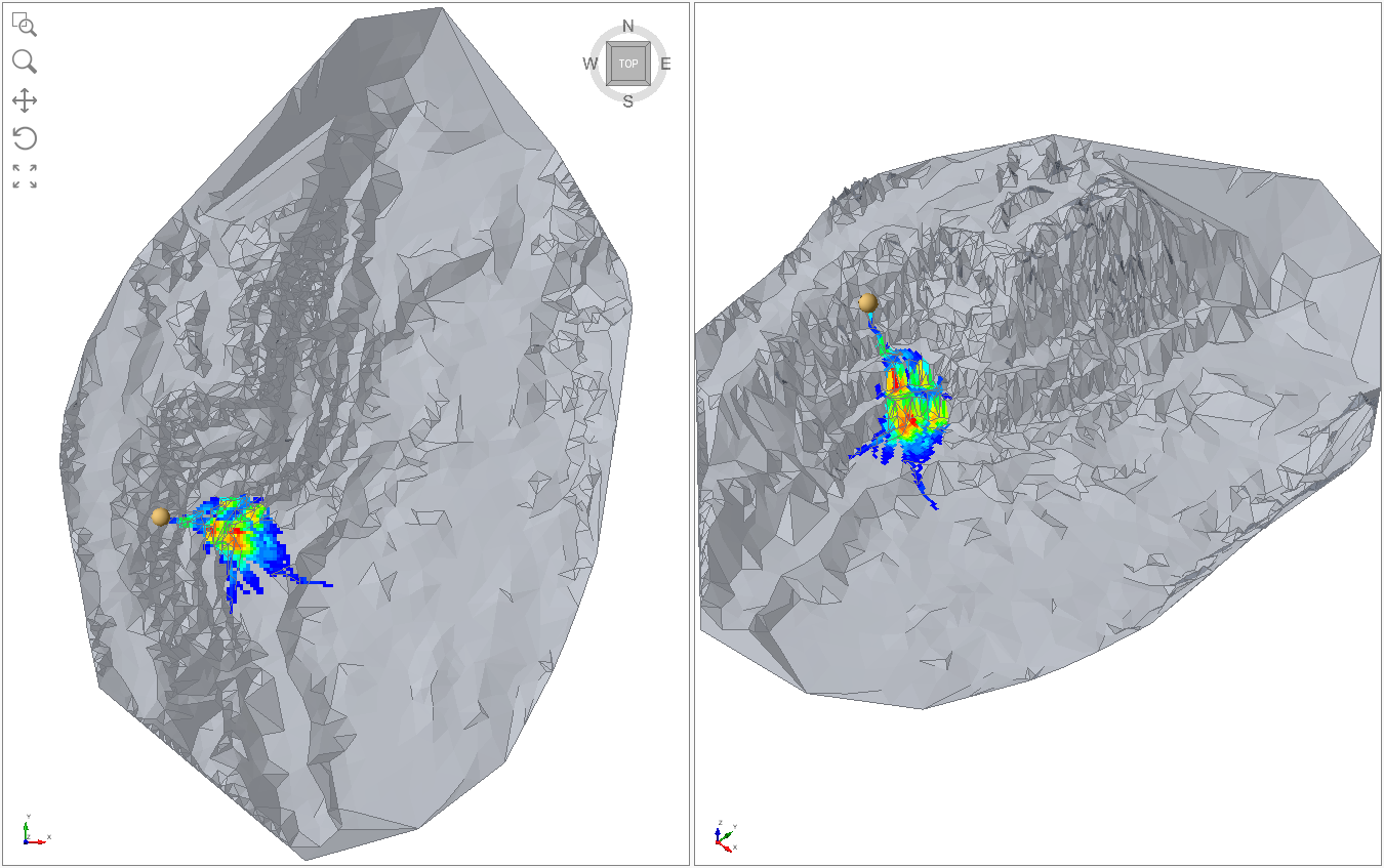
By default, the results displayed are the translational velocities in each rock path, as shown in the legend on the right. Different results may be displayed using the legend options.
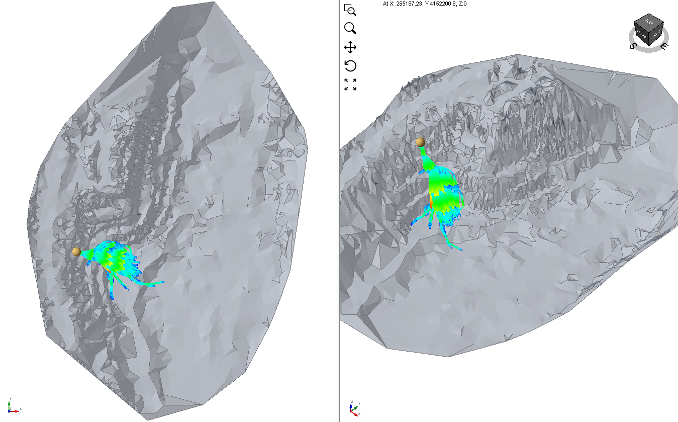
The goal of the analysis is to determine spatially where to place a barrier and to examine the distribution of bounce heights and energies on the barrier to see if there are any critical sections for special consideration.
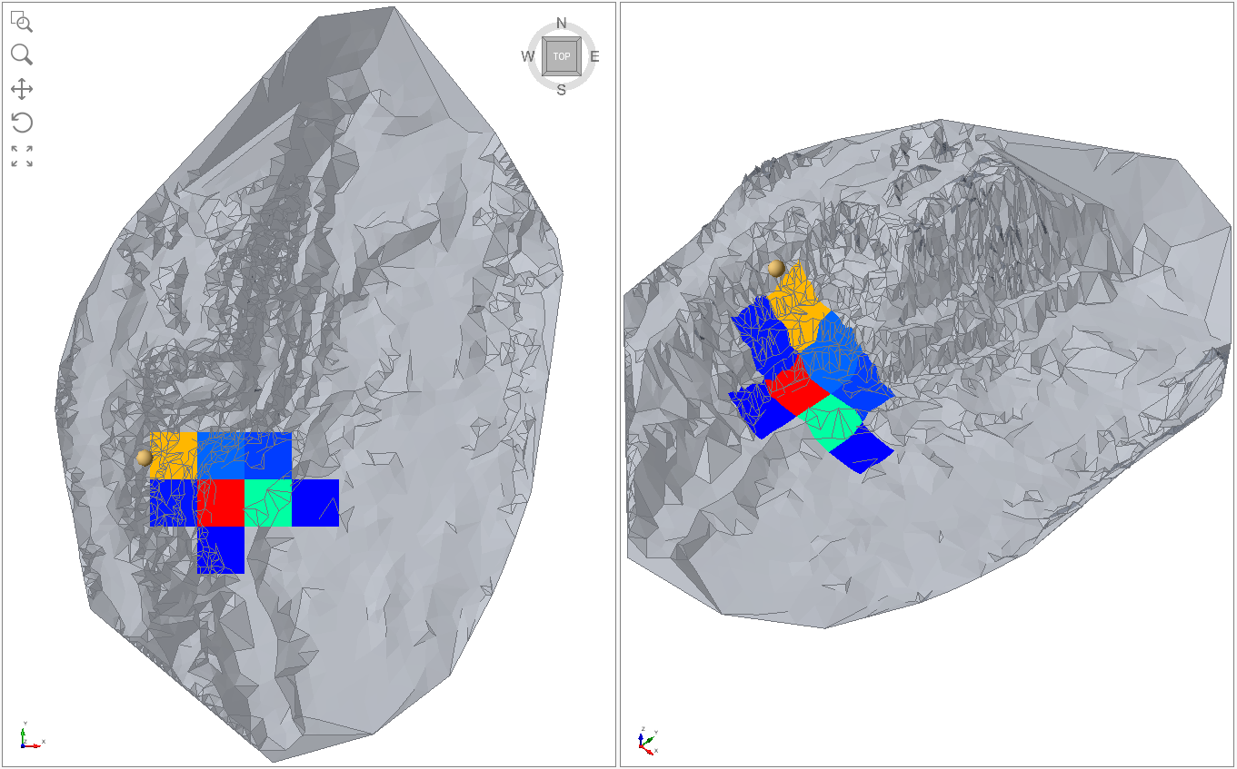
10.1 Heatmap
To help decide on the spatial placement of the barrier, a heatmap of bounce heights and translational kinetic energies can be used to find where barrier installation is feasible (i.e., typically less than 8 m in height and less than 8000 kJ in translational kinetic energy).
To view the surface heatmap:
- Select Interpret > Create Surface Heat Map
 in the main menu or select Surface from the Legend's dropdown menu.
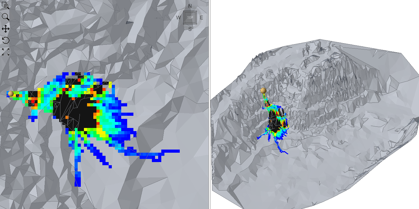
When the heatmap is created, rock paths are displayed in black because the results being displayed are now on the slope surface and not on the rock paths.
- Hide the black rock paths by selecting the 'eye icon' next to Rock Paths in the Visibility Tree.
By default, the Histogram Resolution is set to a minimum of 16.
- Increase the heatmap resolution to a maximum of 256.
- Select Bounce Height from the Data type dropdown menu. The Value Type is "Maximum" meaning that each heatmap grid is displaying the maximum bounce height of all trajectories directly above the grid area. The value type for display can be a maximum, a mean, or a user defined percentile.
Contour settings can be modified to help find areas where the maximum bounce height is less than 8 m.
- Open Contour Options by selecting Interpret > Contour Options

- Choose a Custom Range, and set the range from 0 to 8.
Any area with a maximum bounce height exceeding 8 m would be displayed in black.
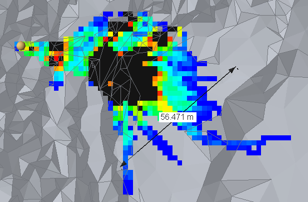
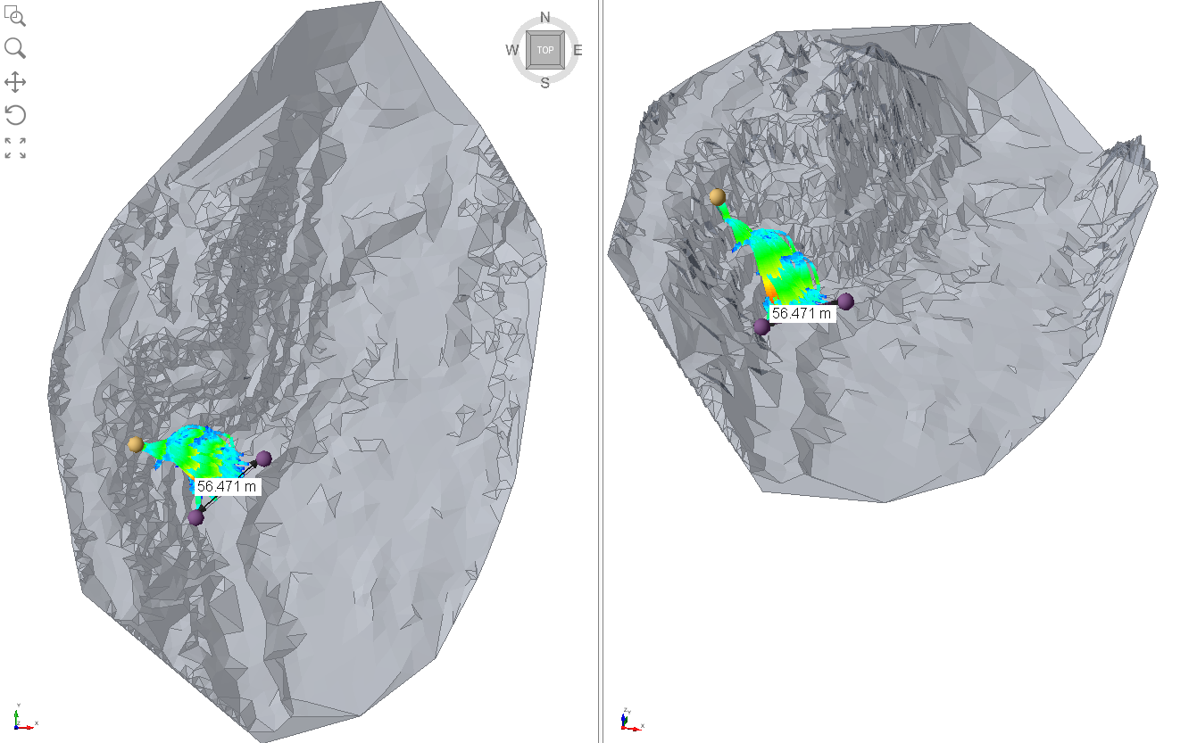
- Before checking the translational kinetic energies, add a smart dimension tool to mark a preliminary barrier placement location. The barrier could be placed where the heatmap shows blue-green or where bounce heights are below 3.5 m.
Check the translational kinetic energy against the capacity available to barriers.
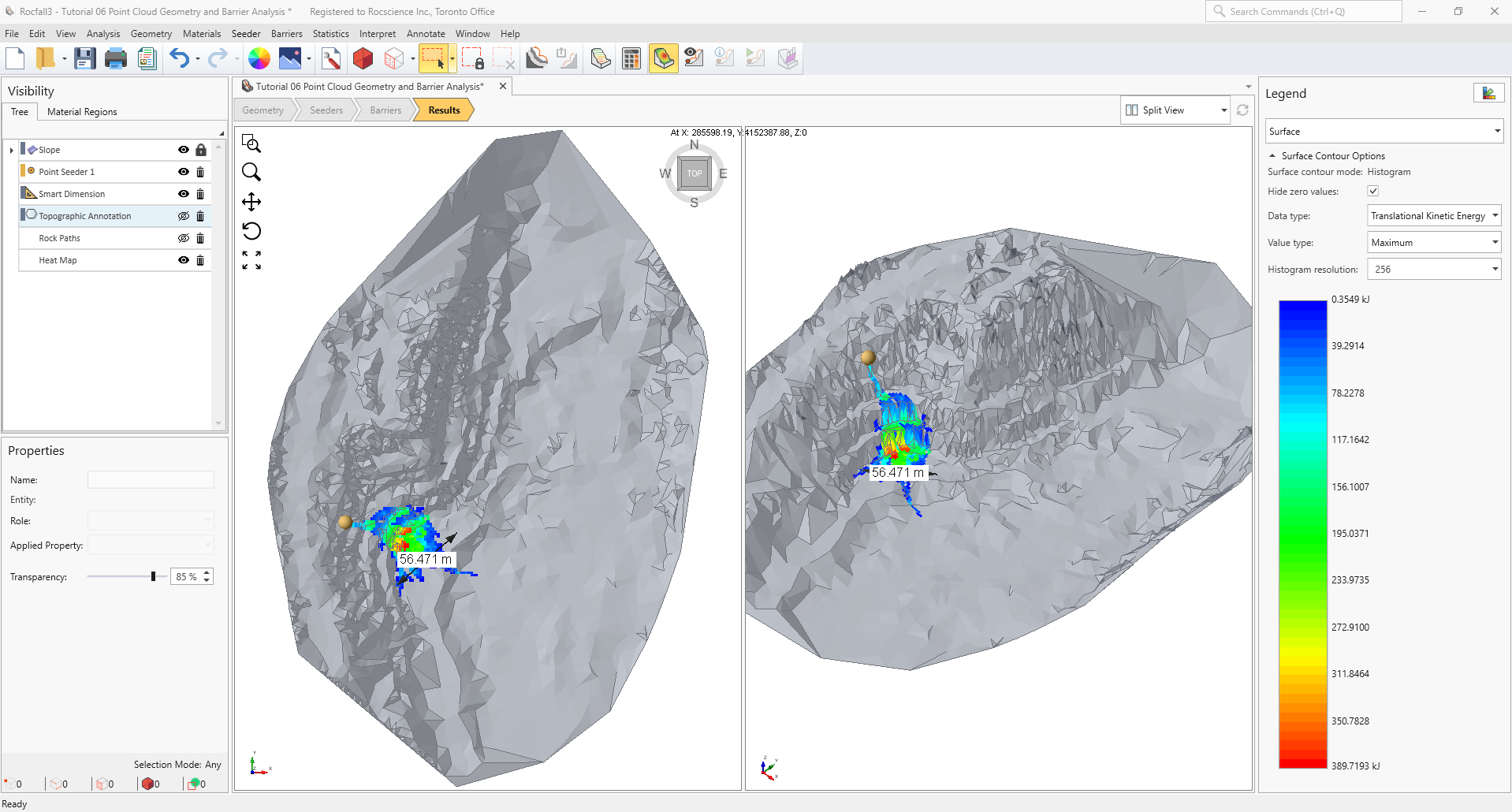
- In the Legend, change the Data type from Bounce Height to Translational Kinetic Energy and open the Contour options
- The auto contour range shows the maximum value for translational energy is only 389 kJ, which is significantly below the 8000 kJ capacity available to the strongest of barriers. Therefore, the bounce height is the governing variable for deciding the placement location of the barrier.
10.2 Barrier Analysis
- Navigate to the Barriers workflow tab and select Barriers > Add Barrier

- Set the height to 3.5 m, and select Add Points on Viewport, left-click for barrier coordinates at each end of the dimensioning tool.
- Select a barrier that has the needed energy level (e.g., 400 kJ) by accessing the barrier properties using the pencil icon

- Save the model and re-compute. Navigate to the Results workflow tab to see whether the barrier provided the protection required.
Examine the distribution of translational kinetic energies and bounce heights on the barrier using the 3D barrier plot.
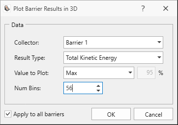
- Select Interpret > Plot Barrier results in 3D
 in the main menu.
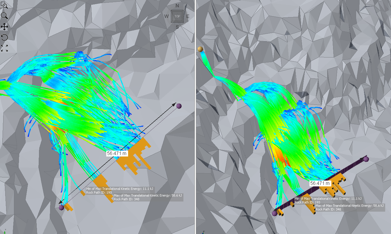
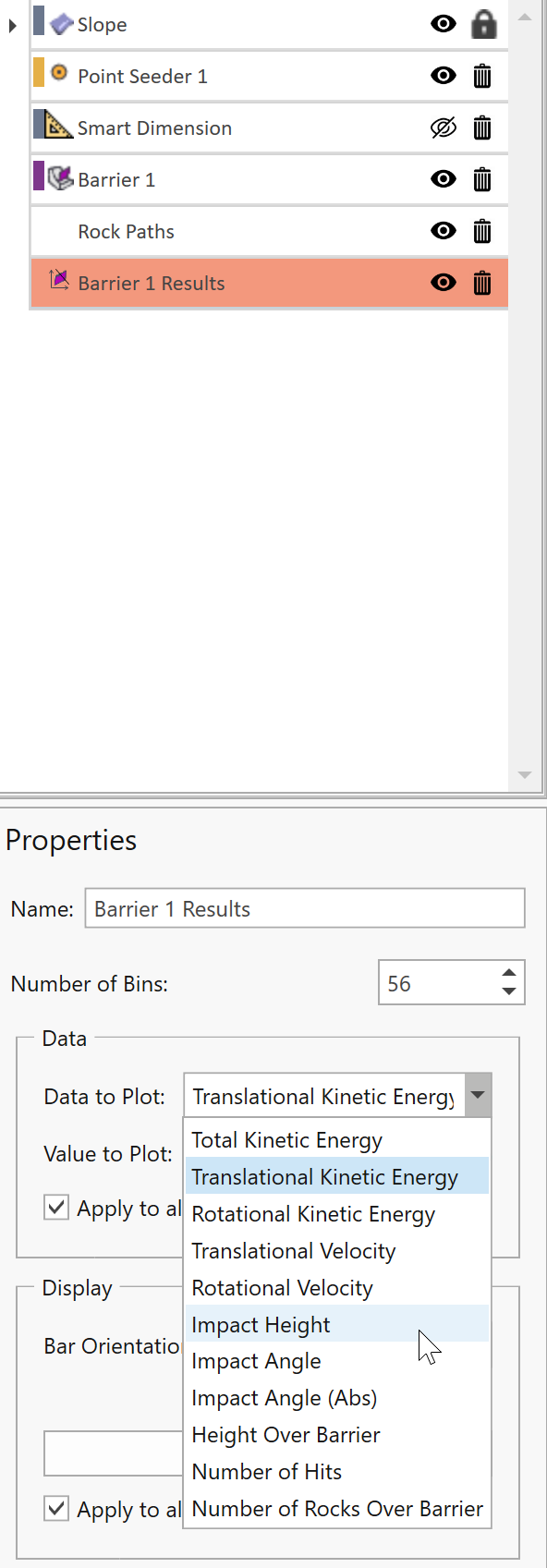
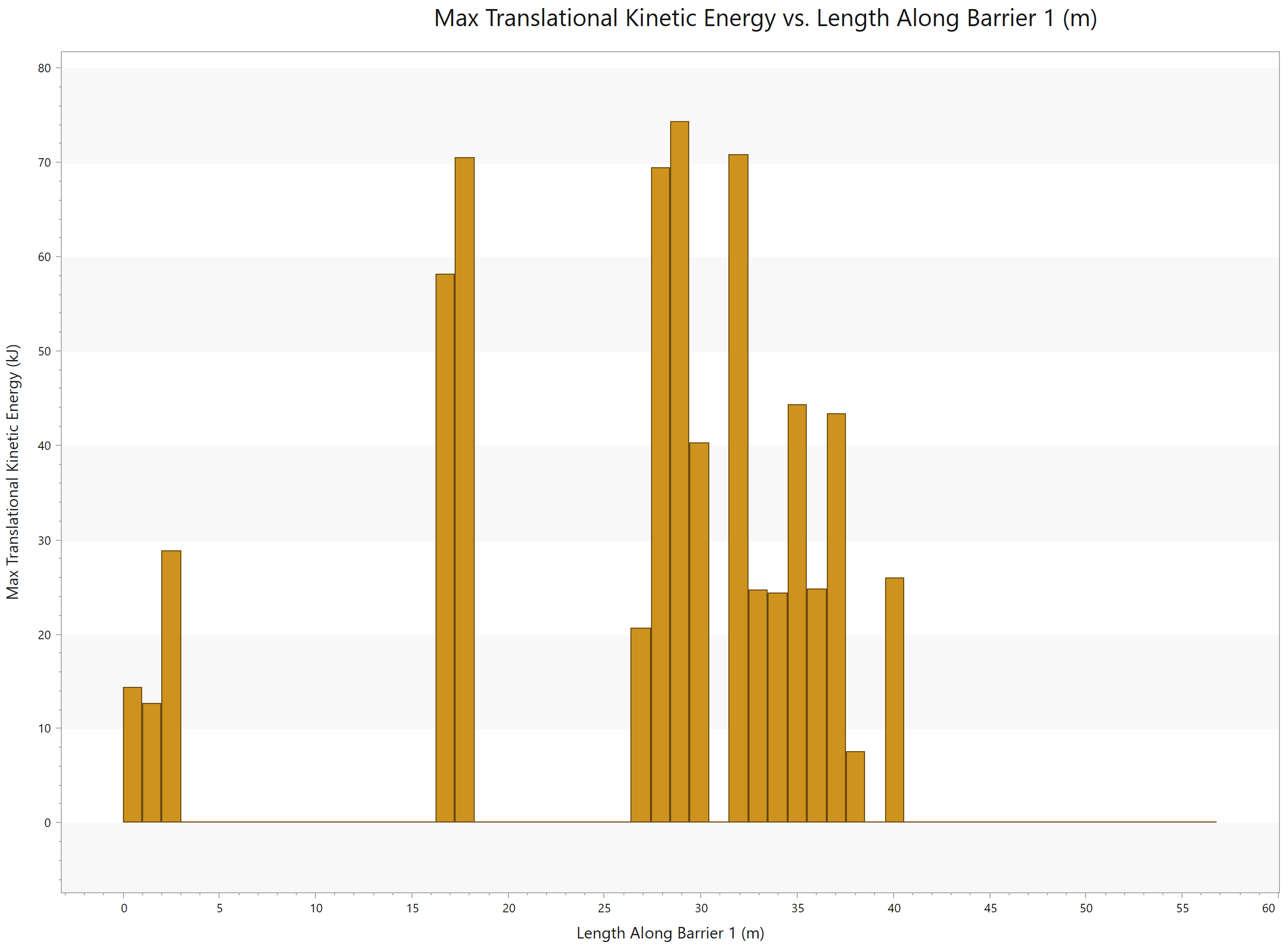
 - Select Barrier 1, change the Result Type to Translational Kinetic Energy, Value to Plot to Max, and change the Num Bins to 56. This creates bins that are approximately 1 m in barrier length.
The distribution of the maximum translational kinetic energy along the barrier is now plotted in the viewports.
- Switch the Data to Plot to Impact Height from the Properties pane.
This will update the 3D barrier plot to show the distribution of rock impact heights along the barrier.
To interpret the value in each bin:
- Select Interpret > Graph Along Barrier

- Set to Barrier 1, change the Result Type to Impact Height and click OK to open the graph.
The distribution of maximum impact heights along the barrier is now shown in a chart view, where the value in each bin can be sampled. The 3D barrier plot and corresponding graph can be used to identify any critical barrier sections and potential 2D slope sections for export to RocFall2.
This concludes Tutorial 6.