5 - Sensitivity & Probabilistic Analysis
1.0 Introduction
This tutorial will demonstrate the process of conducting a Sensitivity Analysis in RocSlope2. A sensitivity analysis allows you to determine the "sensitivity" of the Factor of Safety to variations in the input data. This is done by varying one variable at a time while keeping all other variables constant.
In Tutorial 01 - Quick Start, you learned about the two main analysis types in RocSlope2: Deterministic and Probabilistic, and how to run a Deterministic analysis (the default). In this tutorial, you will learn how to run a Probabilistic analysis.
In a Probabilistic analysis, you can define statistical distributions for input parameters to account for uncertainty in their values. The analysis result is a Factor of Safety distribution from which a Probability of Failure is calculated.
Topics Covered in this Tutorial:
- Sensitivity Analysis
- Probabilistic Analysis
- Random Variables & Statistics
- Histogram Plots
- Scatter Plots
- Cumulative Plots
- Constant and Variable Pseudo-Random Sampling
- Sampling Methods
- Failure Mode Filter
Finished Product:
The finished product of this tutorial can be found in the Tutorial 5 Probabilistic Analysis.rocslope2 file, located in the Examples > Tutorials folder in your RocSlope2 installation folder.
2.0 Importing a RocSlope2 Model File
- If you have not already done so, run the RocSlope2 program by double-clicking the RocSlope2 icon in your installation folder or by selecting Programs > Rocscience > RocSlope2 in the Windows Start menu.
- Select File > New Project

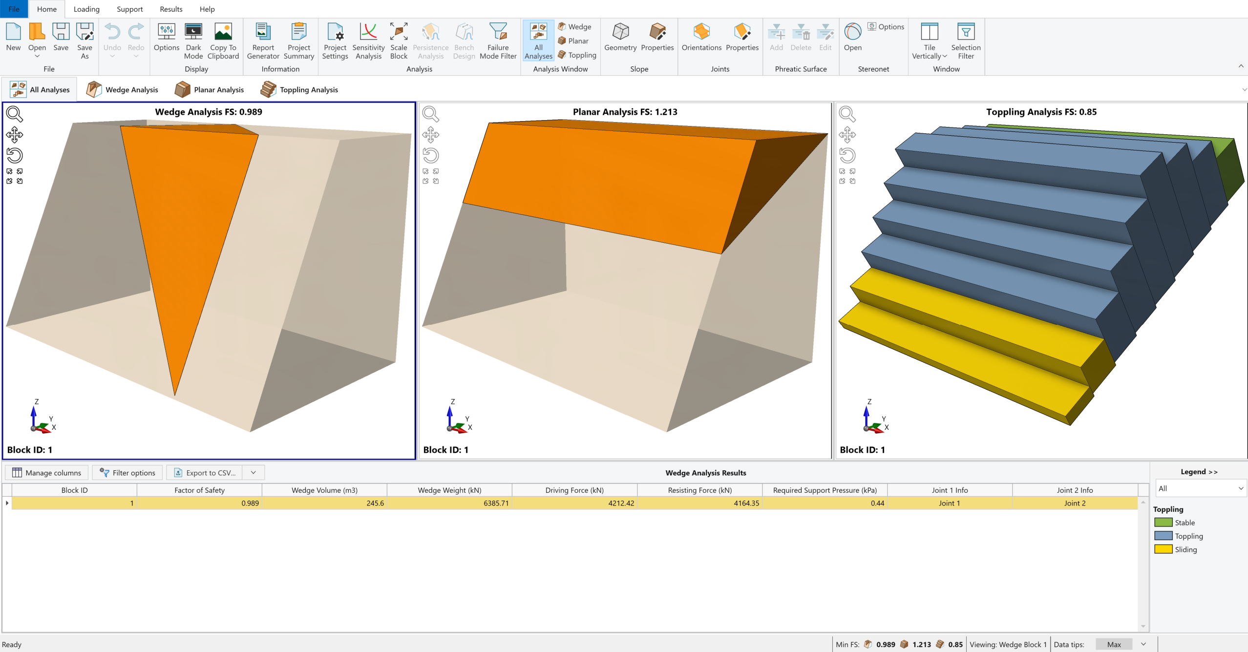
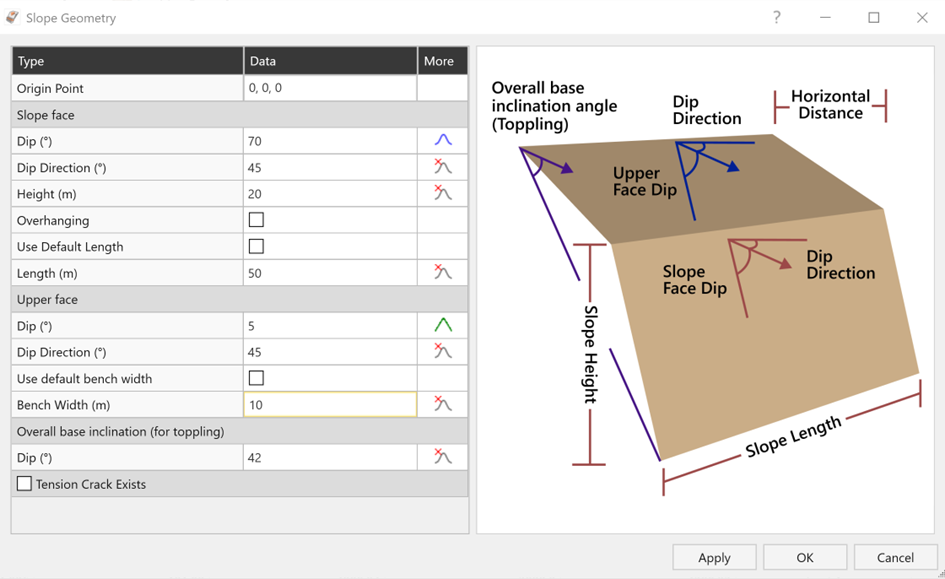
Whenever a new file is created, the default input data forms valid slope geometries for wedge, planar and toppling analysis, as shown in the image below.
This tutorial will use the Tutorial 5 - Sensitivity & Probabilistic Analysis (initial).rocslope2 file as a base model, which is the output model of Tutorial 1 – Quick Start.
- Select File > Open Project

- Open Tutorial 5 - Sensitivity & Probabilistic Analysis (initial).rocslope2 file.
This will open the base file.
3.0 Sensitivity Analysis
In a Sensitivity Analysis, individual variables can be varied among user-defined minimum and maximum values while all other input parameters remain constant for the specified wedge, planar or toppling block. This allows you to determine the effect of individual variables on the Factor of Safety for this block.
3.1 Introduction
The analysis process is as follows:
- The user specifies a minimum and a maximum value for one or more selected input parameters.
- Each parameter is then varied in uniform increments between the minimum and maximum values, and the Factor of Safety of the Global Minimum Slip Surface is calculated at each value. While a parameter is varied, all other input parameters are held constant at their mean values.
- This results in a plot of Safety Factor versus each varied input parameter (a Sensitivity plot) that allows you to determine the “sensitivity” of the Factor of Safety to the variations.
- A steeply changing curve on a Sensitivity plot indicates that the Factor of Safety is sensitive to the value of the parameter.
- A relatively flat curve indicates that the Factor of Safety is not sensitive to the value of the parameter.
- A Sensitivity Plot can also be used to determine the value of a parameter that corresponds to a specified Factor of Safety (e.g. Factor of Safety = 1).
From a practical standpoint, a Sensitivity Analysis in RocSlope2 indicates which input parameters may be critical to the assessment of wedge, planar and/or toppling stability assessment, and which input parameters are relatively less important.
3.2 Model
Variations in the variables for a Sensitivity analysis for each block in each analysis method are set up in the Sensitivity Input dialog. To open the dialog:
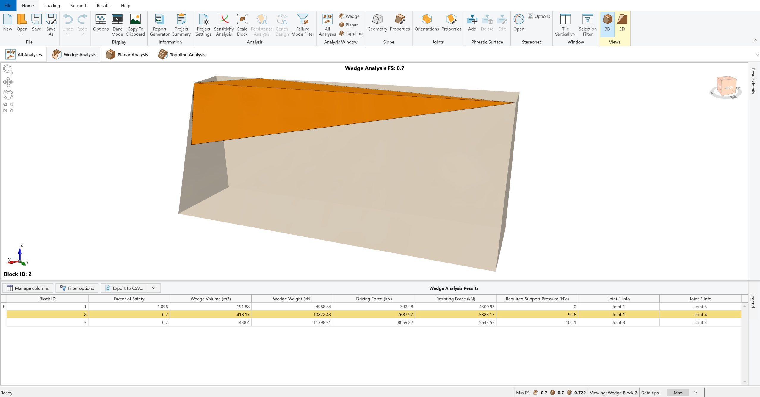
- Double-click on Wedge Analysis pane to open 3D Wedge View.
- Double-click on block with Block ID = 2 to select the block. Notice that wedge is formed by the intersection of Joint 1 and Joint 4.
- Select Home > Analysis > Sensitivity Analysis

- Click on the dropdown menu in the Type column and select Joint 4 Cohesion (kPa).
- Set From and To values as follows:
- From = 0
- To = 10
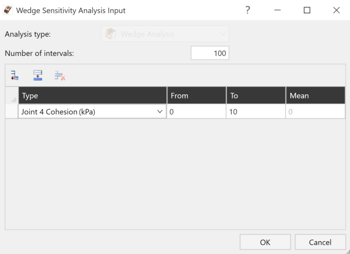
- From = 0
- Click OK to accept the changes and automatically plot the Sensitivity Plot for defined Joint 4 Cohesion (kPa) range.
Notice that the following Sensitivity Plot is generated automatically under the Sensitivity View tab for defined Joint 4 Cohesion (kPa) range.
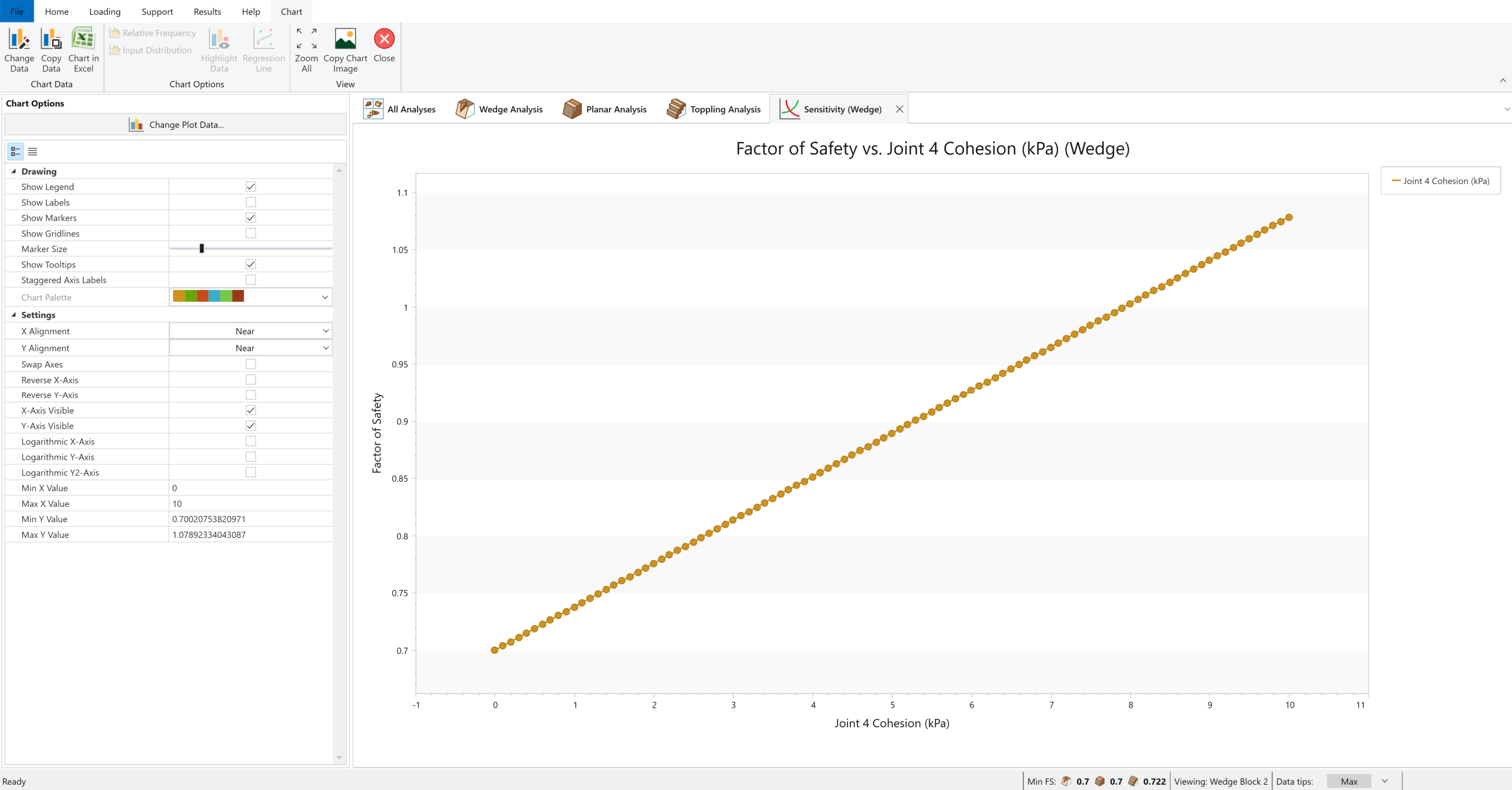
You can see that the Factor of Safety is increasing with the increase of Joint 4 Cohesion (kPa), as expected, since the shear strength along Joint 4 is increasing.
Close the Sensitivity Plot by clicking the X on the Sensitivity View tab or Close  icon on the toolbar.
- Double click on anywhere off the model in 3D Wedge View to restore the All Analyses View.
3.3 Multi-Variable Sensitivity Analysis
- Double click on Toppling Analysis pane to open the 3D Toppling View.
- Select Home > Analysis > Sensitivity Analysis
- Click on the drop down menu in the Type column and select Slope Face Dip (°).
- Set From and To values as follows:
- From = 55
- To = 80
- From = 55
- Click Add Single Row
 to add another Sensitivity Analysis Input.
 - Click on the dropdown menu in the second row of Type column and select Overall Base Inclination Dip (°).
- Set From and To values as follows:
- From = 30
- To = 50

- From = 30
- Click OK to accept the changes and automatically plot the Sensitivity Plot for defined Slope Face Dip (°) and Overall Base Inclination Dip (°) variable in the same graph.
Notice that the following Sensitivity Plot is generated automatically under Sensitivity View tab for defined Slope Face Dip (°) and Overall Base Inclination Dip (°) variable in the same graph. The graph will now display two curves.
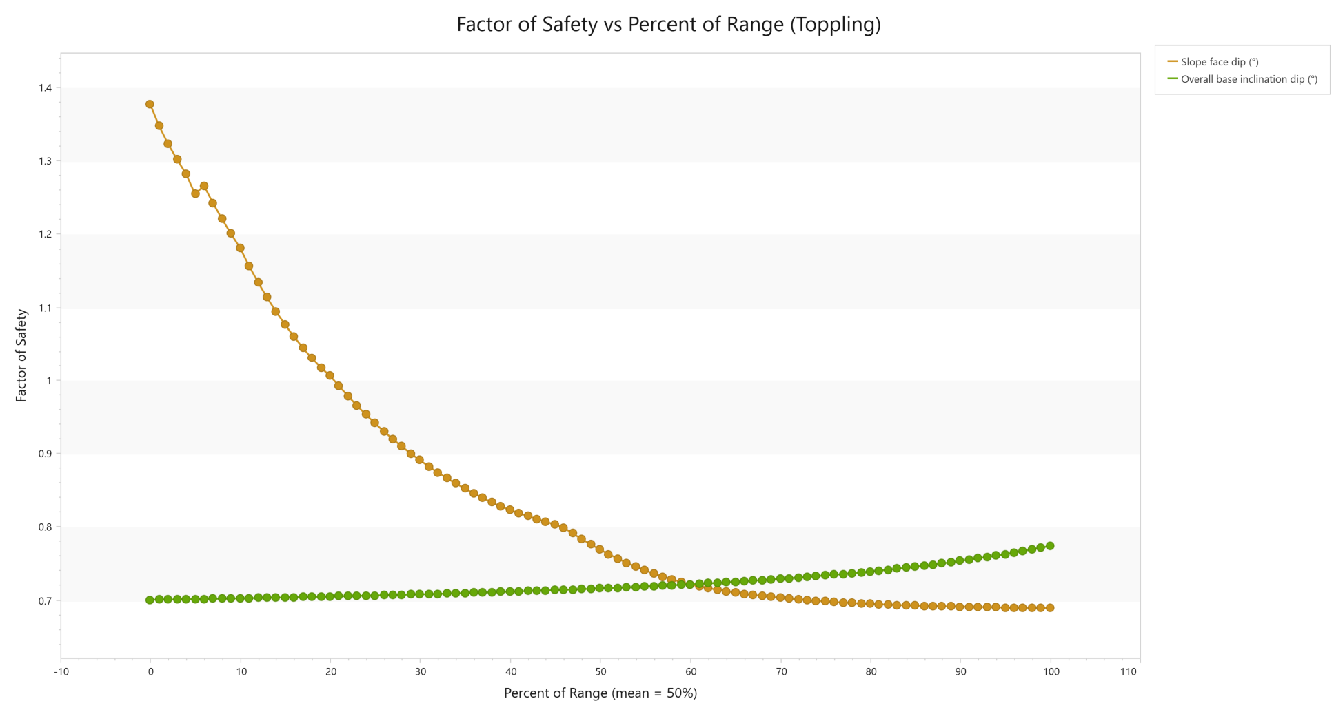
You can see that the Factor of Safety is decreasing with the increase of Slope Face Dip (°) while it is increasing with the increase in Overall Base Inclination Dip (°). The effect of Slope Face Dip (°) on the Factor of Safety is relatively higher than Overall Base Inclination Dip (°) since it has a relatively steeply changing curve on the Sensitivity plot.
- In the Sensitivity Analysis Input dialog, the From and To values can be user-defined.
- There is no limit to the number of Sensitivity Analysis Inputs to be defined.
- The Mean value of each variable is determined from the Input Data dialog and CANNOT be changed in the Sensitivity Input dialog.
- When more than one input data variable is plotted on a Sensitivity plot, the horizontal axis is in terms of Percent of Range rather than the actual variables. The Percent of Range is the relative difference between the minimum (From) value of a variable (0 percent) and the maximum value (To) of a variable (100 percent).
Note the following additional learning points:
- Notice that Chart Options are available in the left sidebar in Sensitivity View. The Chart Options sidebar allows you to customize chart axes and colours.
- Chart Data or the Chart Image can be copied by clicking the Copy Data
 or Copy Chart Image
  buttons on the toolbar (or by right-clicking in the chart and selecting corresponding option).
 - Chart data can be exported and graphed in Excel. The Chart in Excel
 option is available in the toolbar or the right-click menu.
Close the Sensitivity Plot by clicking the X on the Sensitivity View tab or Close icon on the toolbar.
- Double click on anywhere off the model in 3D Toppling View to restore the All Analyses View.
4.0 Probabilistic Analysis
In a Probabilistic analysis, statistical input data can be entered to account for uncertainty in slope geometry, joint orientation, strength values, support forces, seismic force and point of force application. The result is a distribution of Factors of Safety, from which a Probability of Failure is calculated. To learn more about Probabilistic Analysis, see the Probabilistic Analysis Overview topic.
4.1 Project Settings
The Project Settings dialog allows you to configure the main analysis parameters for your model, such as Analysis Method, Analysis Type and Units. To open the dialog:
- Select Home > Analysis > Project Settings

4.1.2 Units
- Under the Units
 tab, ensure Units = Metric, stress as kPa.
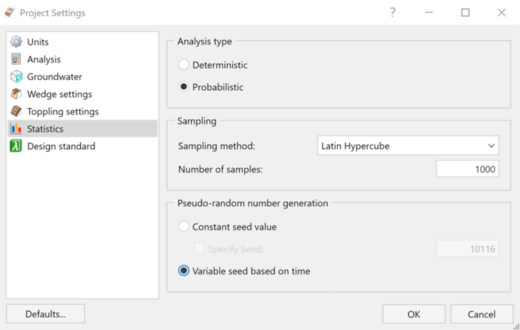
4.1.3 Statistics and Analysis Type
- Select the Statistics
 tab.
tab. - Set Analysis Type = Probabilistic.
- Ensure Sampling Method = Latin Hypercube and Number of Samples = 1000.
- Under Pseudo-random number generation, ensure Constant seed value is selected
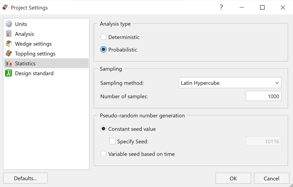
The Sampling Method determines how the statistical distribution for the random input variables will be sampled. The default settings are Sampling Method = Latin Hypercube and Number of Samples = 1000. For detailed information, see the Statistics topic.
Note that Pseudo-Random Number Generation is set to Constant seed value by default. This allows you to obtain reproducible results for a probabilistic analysis by using the same seed value to generate random numbers. We will discuss Constant versus Variable seed options later in this tutorial.
4.1.4 Analysis and Design Factor of Safety
- Select the Analysis
 tab.
tab. - Ensure the Design Factor of Safety is set to 1.
- Ensure all Analysis Methods are selected.
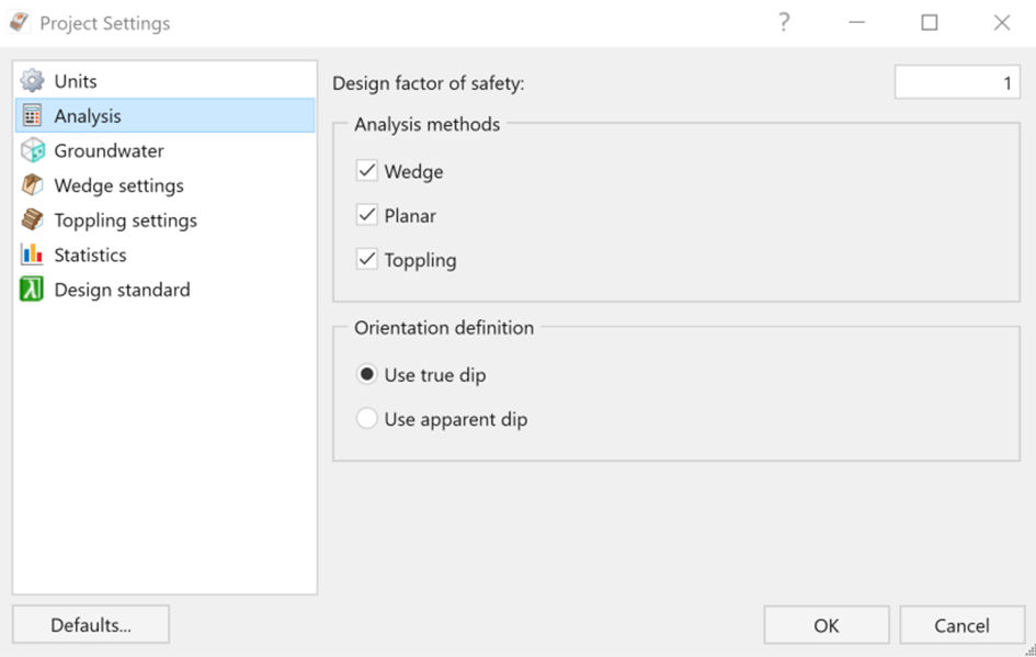
- The Design Factor of Safety option is used in Probabilistic analysis to determine both the Probability of Failure and the number of failed wedges in graphs. The Probability of Failure is now P(FS < Design FS).
- Click OK to apply the changes and close the Project Settings dialog.
4.2 Probabilistic Input Data
To carry out a Probabilistic analysis with RocSlope2, at least one input parameter must be defined as a random variable. To define a random variable, you select a statistical distribution (e.g., Normal, Lognormal, Fisher, etc.) for the variable and enter appropriate parameters (e.g., Standard Deviation, Relative Minimum, Relative Maximum, etc.).
Now we will define the random variables for the Probabilistic analysis. This is done through corresponding dialogs such as Slope Geometry, Slope Properties, Joint Orientations, Joint Properties, etc. for each random variable to be defined.
For the example in this tutorial, we will define the following input parameters as random variables:
- Slope Face Dip
- Upper Face Dip
- Joint Property 1 strength (Phi)
- Joint Property 2 strength (Cohesion and Phi)
- Joint Orientations
All other input parameters are assumed to be exactly known (i.e., Statistical Distribution = None) and will not be involved in the statistical sampling.
4.2.1 Slope Face Dip
- Select Home > Slope > Geometry

- Click on Statistical Distribution
 icon next to Slope Face Dip to open the statistical distribution dialog.
 - Enter the following:
- Distribution = Normal
- Standard Deviation (Std. Dev.) = 3
- Relative Minimum (Rel. Min.) = 9
- Relative Maximum (Rel. Max.) = 9
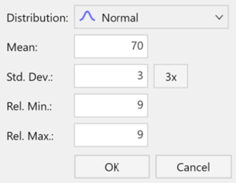
- Click OK to apply the changes and close the dialog.
4.2.2 Upper Face Dip
- Click on the Statistical Distribution icon next to Upper Face Dip to open the statistical distribution dialog.
- Set Distribution = Triangular
- Set Relative Minimum (Rel. Min.) = 2 and Relative Maximum (Rel. Max.) = 2.
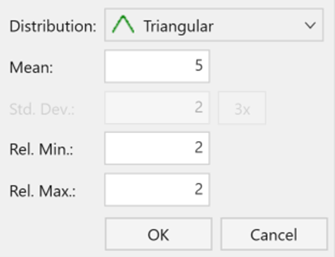
- Click OK to apply the changes and close the dialog.
- Ensure Use Default Bench Width option is unchecked and set Bench Width (m) = 10.
- Click OK to apply the changes and close the Slope Property dialog.
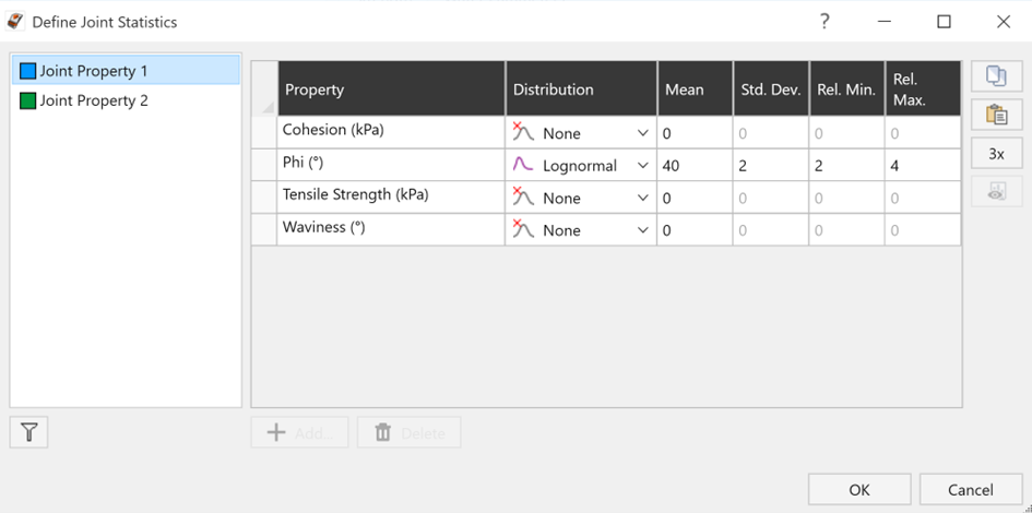
4.2.3 Joint Property 1 Strength
- Select Home > Joints > Properties

- Select Statistics to define statistics for all properties. This will open Define Joint Statistics dialog.
- Ensure that Joint Property 1 is selected in Define Joint Statistics dialog.
- Set Mean Phi () = 40.
- Set Distribution = Lognormal next to Phi () and enter the following values:
- Standard Deviation = 2
- Relative Min. = 2
- Relative Max. = 4
- Standard Deviation = 2
4.2.4 Joint Property 2 Strength
- Select Joint Property 2 in Define Joint Statistics dialog.
- For Cohesion (kPa), set Distribution = Lognormal and enter following values:
- Standard Deviation = 1
- Relative Min. = 2
- Relative Max. = 3
- For Phi (°), set Distribution = Lognormal and enter following values:
- Standard Deviation = 2
- Relative Min. = 2
- Relative Max. = 6
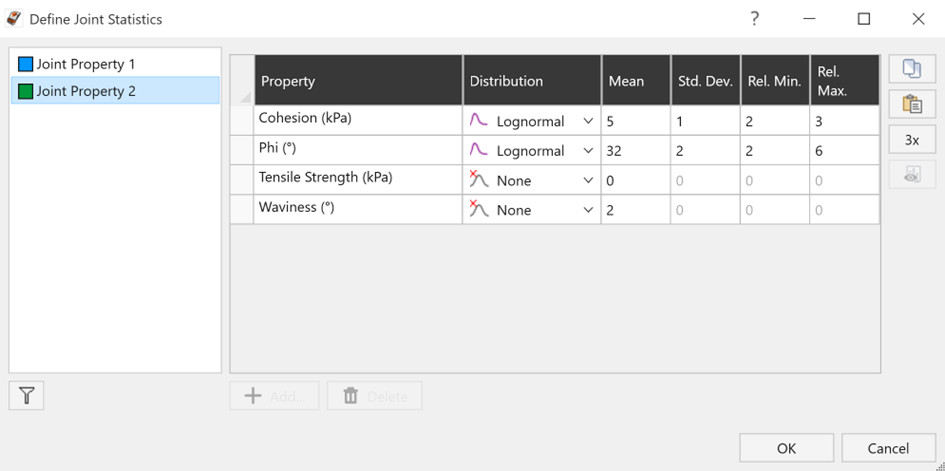
- Click OK to apply the changes and close the Define Joint Statistics dialog.
- Joint Property 1 and Joint Property 2 strength random variables are now defined.
- Click OK to apply the changes and close the Define Joint Properties dialog.
4.2.5 Joint Orientations
- Select Home > Joints > Orientations

Note that there are two methods of defining the variability of joint orientation (Orientation Definition Method):
- Dip/Dip Direction: The Dip and Dip Direction are treated as independent random variables (i.e., you can define different statistical distributions for each one).
- Fisher Distribution: Generates a symmetric, three-dimensional distribution of orientations around the mean plane orientation, so only a single standard deviation is required. In general, a Fisher Distribution is recommended for generating random joint plane orientations because it provides more predictable orientation distributions and lessens the chance of input data errors.
For this tutorial, we are using the Fisher Distribution option.
- Set Orientation Definition Method = Fisher.
- Set Fisher Option = Standard Deviation.
- Set Joint Standard Deviations as follows:
- Joint 1 Standard Deviation = 0
- Joint 2 Standard Deviation = 7
- Joint 3 Standard Deviation = 0
- Joint 4 Standard Deviation = 4
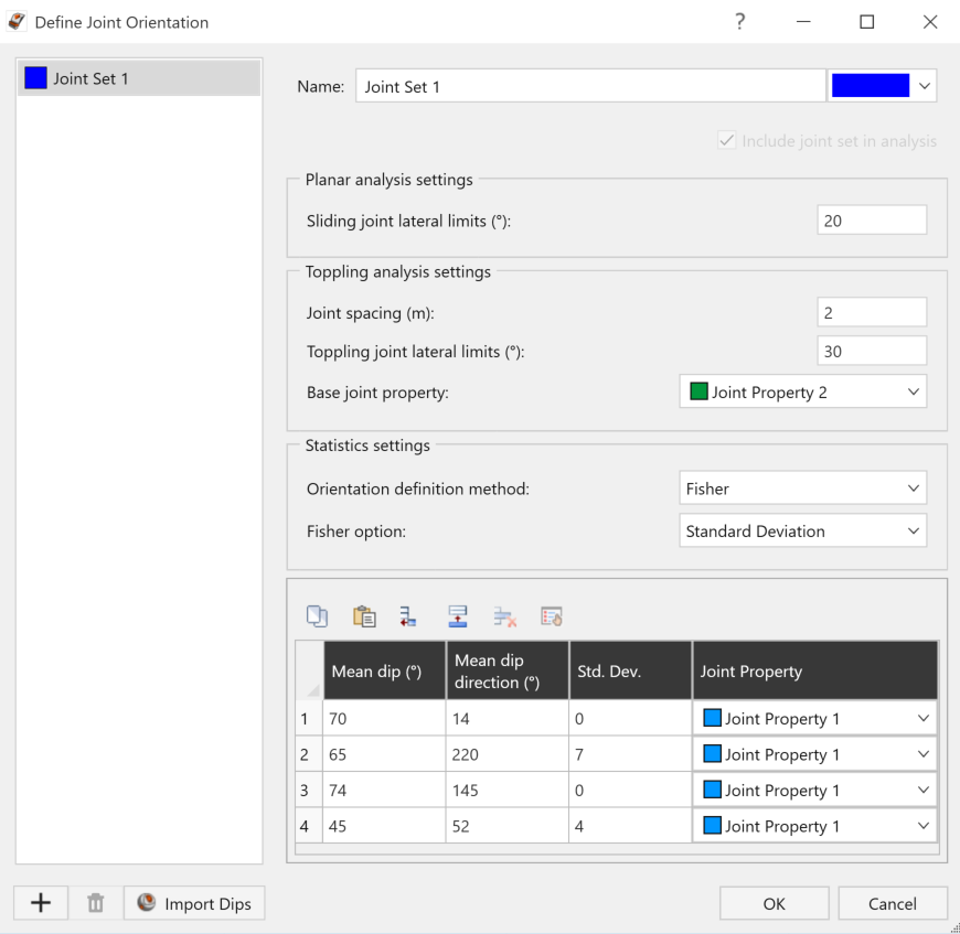
- Joint 2 and Joint 4 orientation random variables are now defined.
- Click OK to apply the changes and close the Define Joint Orientation dialog.
5.0 Probabilistic Analysis Results
To ensure the latest analysis results are always displayed, RocSlope2 automatically computes an analysis whenever an input data is entered or modified in a dialog and Apply or OK is clicked. Notice that the Probability of Failure (PoF) for Wedge, Planar and Toppling analyses are computed instantly considering current input data and defined random variables.
5.1 Probability of Failure
The primary result of interest from a Probabilistic analysis is the Probability of Failure (PoF). Probability of Failure value for each analysis method will be automatically displayed at the top of corresponding analysis pane (at the title bar) in the split-screen view.
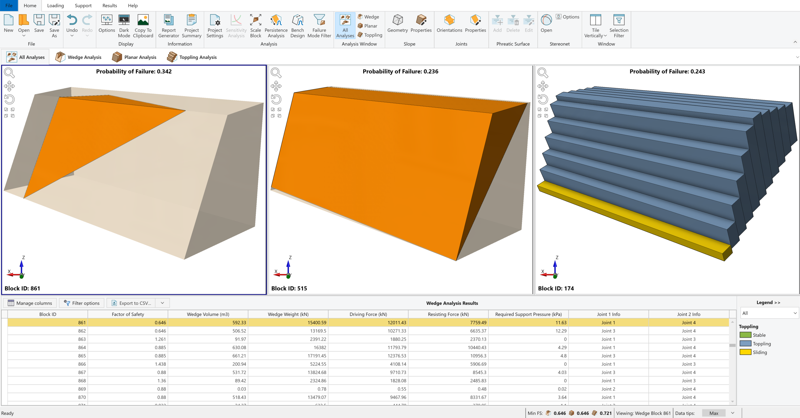
If you entered the input data correctly, you should obtain a Probability of Failure of about 34.2% (0.342) for Wedge Analysis, Probability of Failure of about 23.6% (0.236) for Planar Analysis and Probability of Failure of about 24.3% (0.243) for Toppling Analysis.
Note that the Probability of Failure is equal to the Number of Failed Wedges (i.e., those with a Factor of Safety < Design Factor of Safety) divided by the Total Number of Possible Wedges that can be generated in a probabilistic combination analysis, i.e., 2049 / 6000 for Wedge analysis, 943 / 4000 for Planar analysis, 972 / 4000 for Toppling analysis in this tutorial.
5.2 Histograms
Now let's plot a histogram of the Probabilistic analysis results, using the Histogram dialog. To plot histograms of results after a Probabilistic analysis:
- Select Results > Charts > Histogram
- The Analysis Type is set to the current Analysis Pane selection and the Data to Plot is set to Factor of Safety by default.
- Set the Analysis Type = Planar Analysis.
- Leave Number of Bins = 30.
- Select the Highlight Data checkbox and leave the Factor of Safety to <1.
- Click OK.
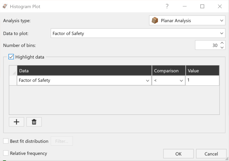
A histogram of the Factor of Safety is displayed in the Histogram View.
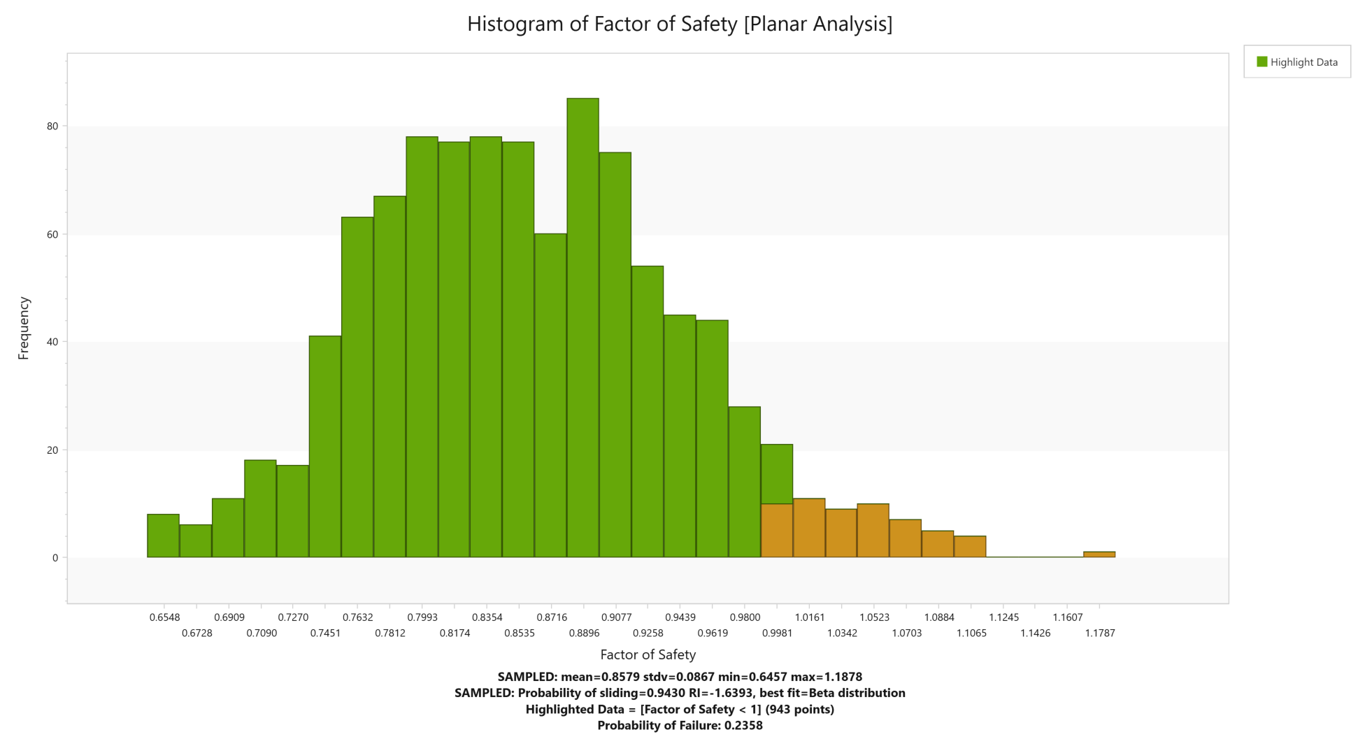
The histogram represents the distribution of the Planar Analysis Factor of Safeties for all valid blocks generated by random sampling based on data entered in the input data dialogs. The green bars to the left represent blocks with a Factor of Safety of less than 1.0 while the orange bars to the right represent blocks with a Factor of Safety greater than 1.0. This allows you to see the relationship between failed block (block with Factor of Safety < Design Factor of Safety) and the distribution of any input or output variable.
5.2.1 Mean Factor of Safety
Notice the values displayed at the bottom of the histogram for the mean Factor of Safety, the standard deviation, and the minimum and maximum values.
The mean Factor of Safety from a Probabilistic analysis (i.e., the average of all the Factors of Safety generated by the analysis) is generally slightly different from the Factor of Safety of the Mean Wedge (i.e., the Factor of Safety of the wedge corresponding to the mean values entered in the Input Data dialog). You can view the Safety Factor of the Mean Wedge in the Results tab for each analysis method, by selecting the Show Mean FS Result  option.
For this tutorial, these values are:
- The mean Factor of Safety for Planar Analysis (from the histogram) = 0.858
- The Factor of Safety of the Mean Wedge for Planar Analysis (from the Results Grid) = 0.839
Theoretically, for an infinite number of samples, these two values should be equal. However, due to the random nature of the statistical sampling, the two values are usually slightly different for a typical probabilistic analysis with a finite number of samples.
5.2.2 Histograms of Other Data
In addition to the Factor of Safety, you can plot histograms of various data (i.e. wedge information, forces, stresses, slope geometry, etc.). This can be easily done in the Histogram Plot View.
- Select Change Plot Data on the left sidebar in Histogram Plot View.
- Set Analysis Type = Planar Analysis.
- Set Data to Plot = Failure Plane Angle (°).
- Select the Best Fit Distribution check box.
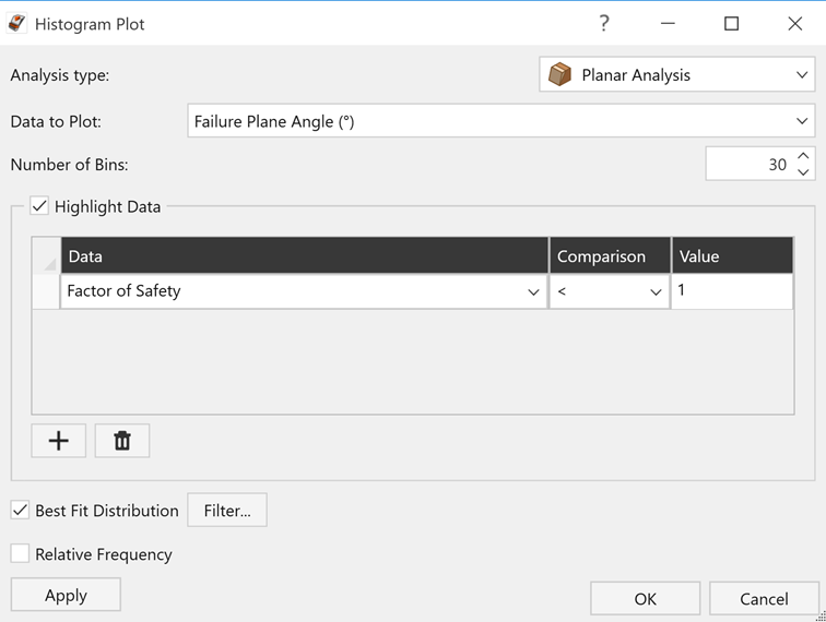
- Click OK.
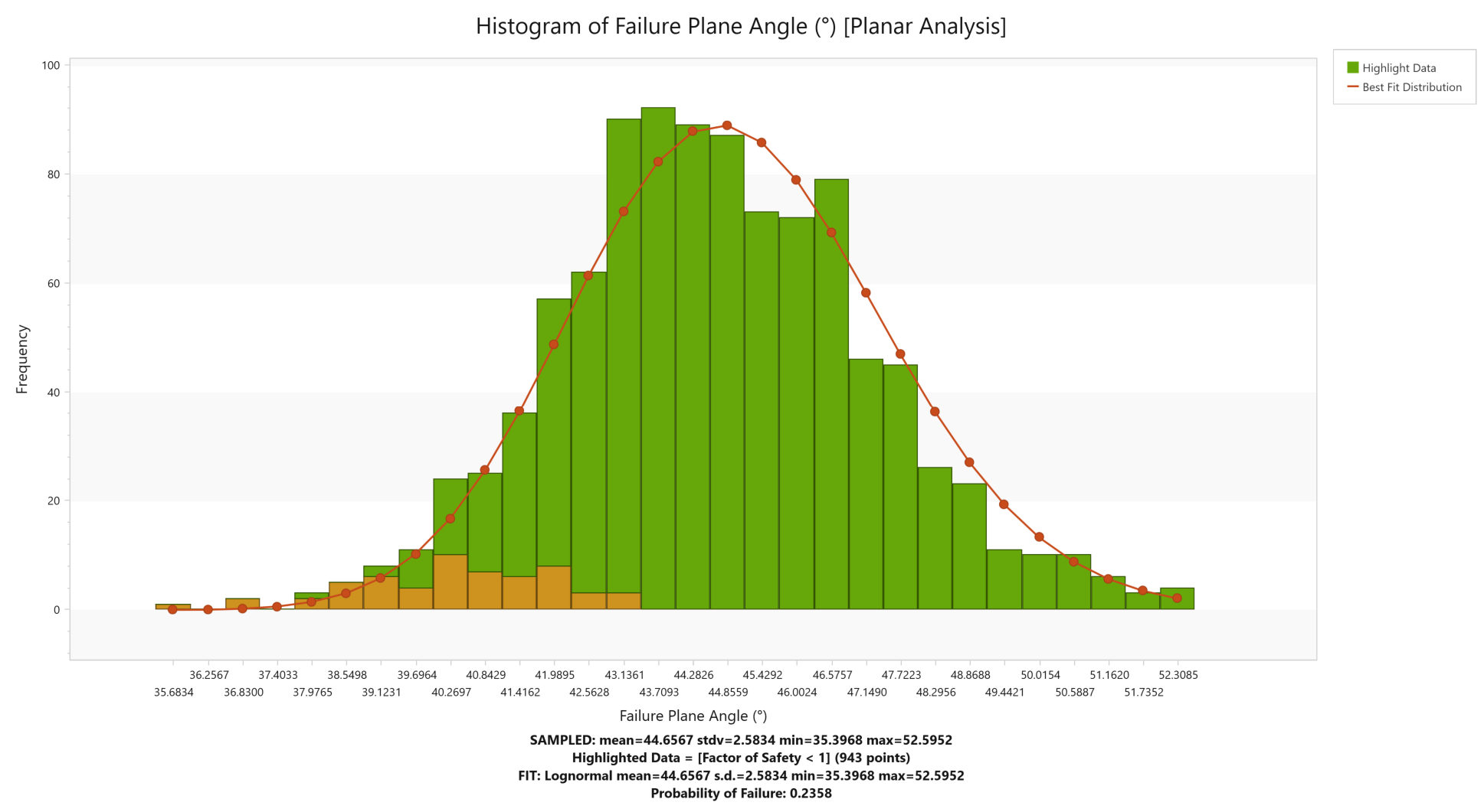
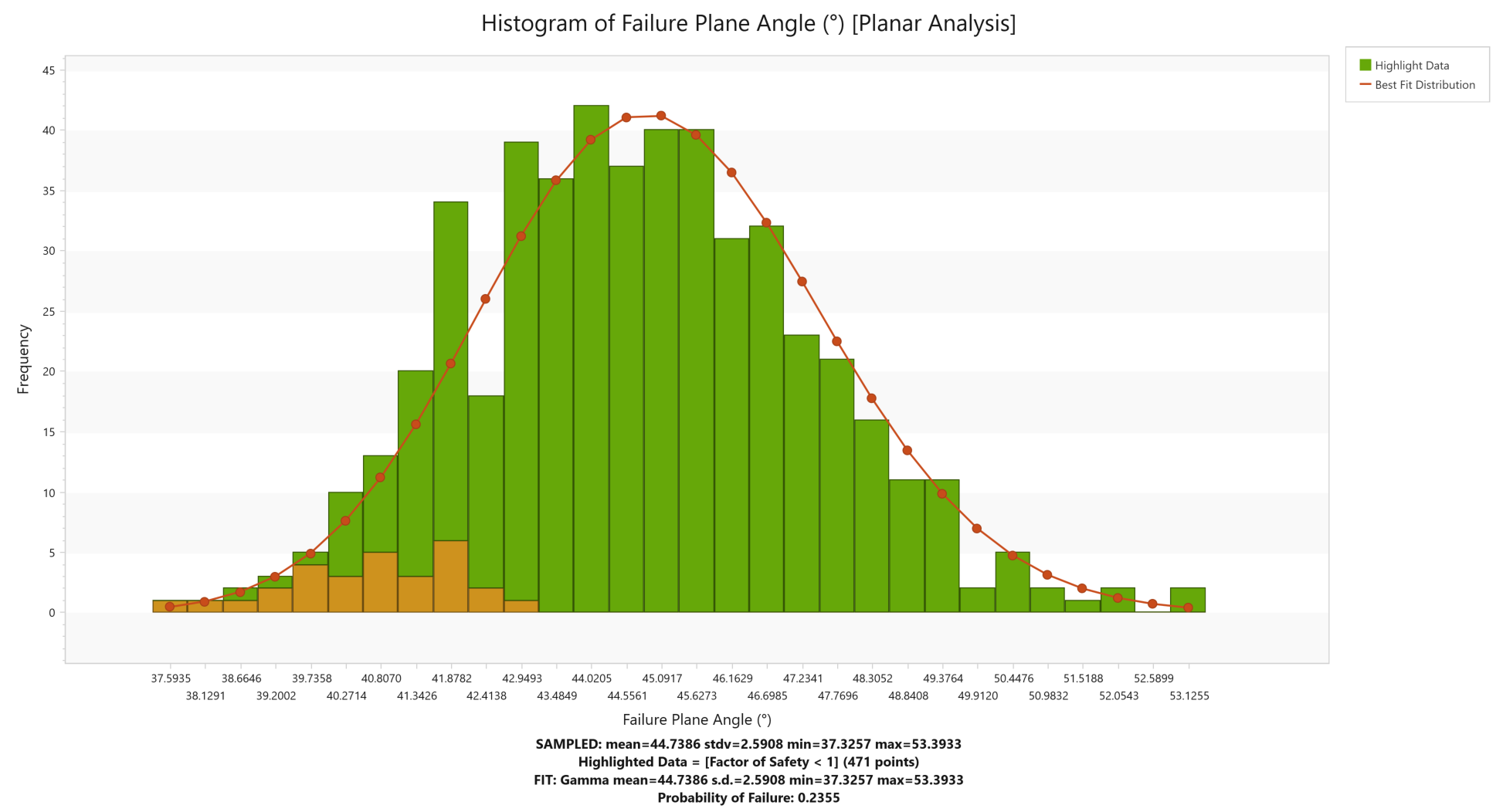
A histogram of the Failure Plane Angle (°) distribution is generated for Planar Analysis, as shown below.

In this case, the Best Fit Distribution is a Lognormal distribution, and the corresponding parameters are displayed at the bottom. All features of the Safety Factor histogram described above also work for this and other data types.
This histogram shows us the failed blocks correspond to blocks with steeper Failure Plane Angles (°), as can be seen above.
Now let's generate one more histogram. This time we'll plot one of the input data random variables.
- Select Change Plot Data on the left sidebar in Histogram Plot View.
- Set Analysis Type = Wedge Analysis.
- Set Data to Plot = Slope Dip (º).
- Ensure Input Distribution checkbox is selected.
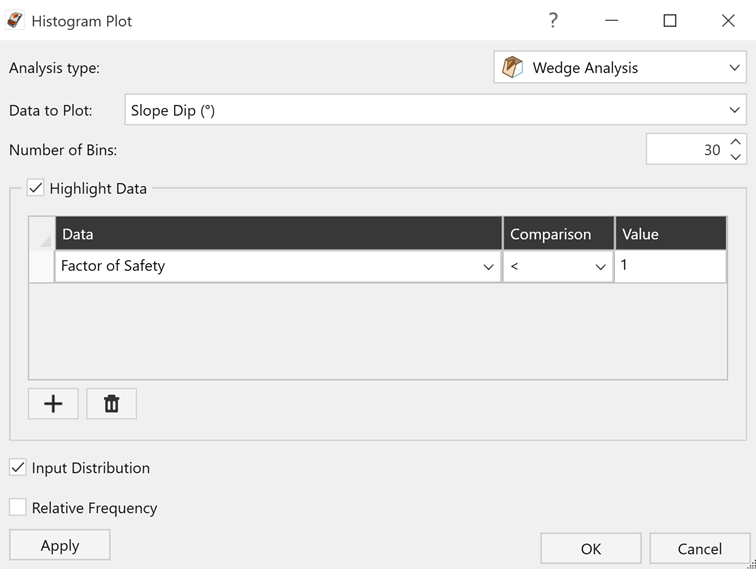
- Click OK.
A histogram of the Slope Dip (°) distribution is generated for Wedge Analysis, as shown below.
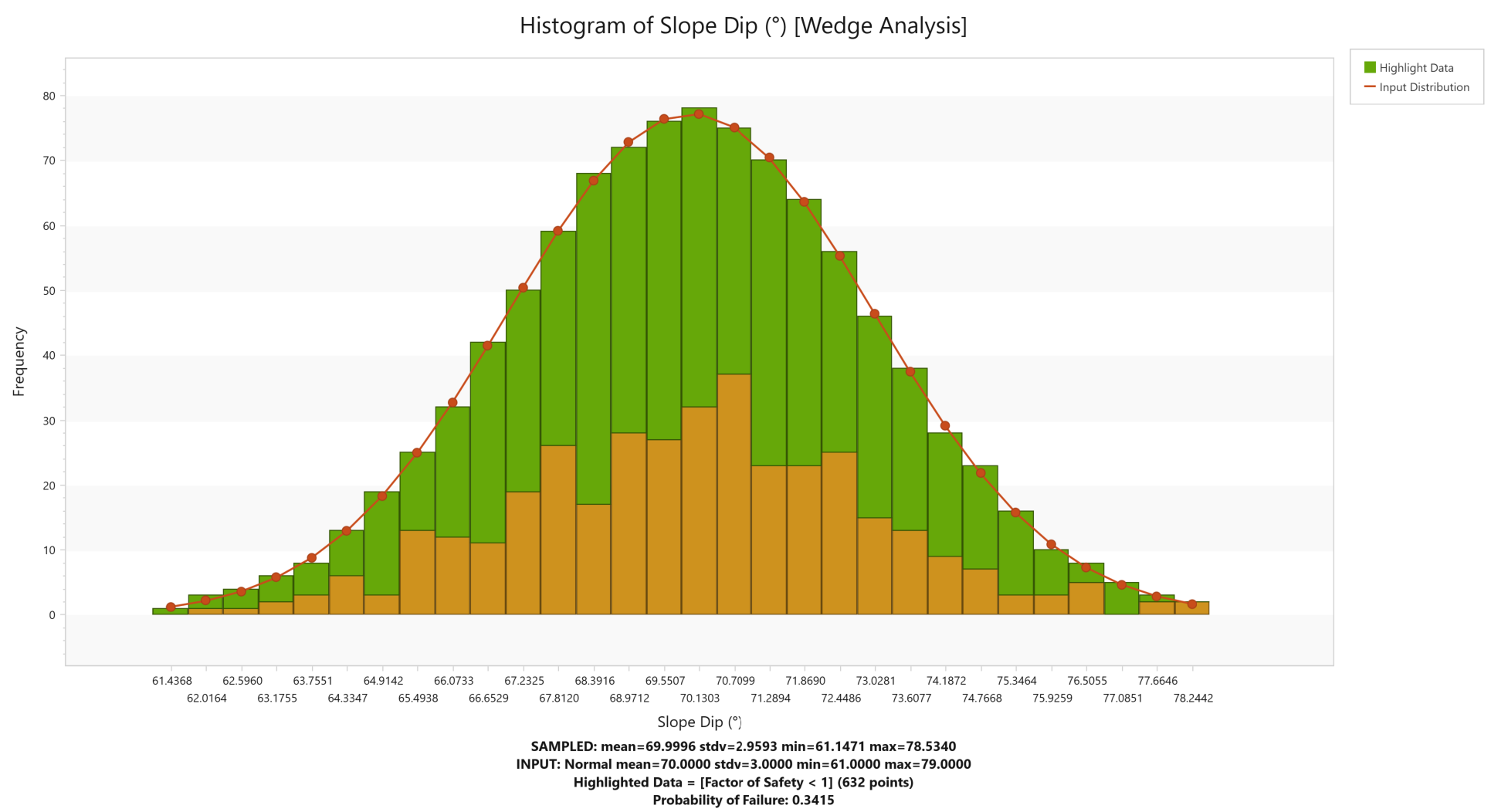
Notice that the Input Distribution is Normal distribution as we entered for Slope Dip (°) variable and the input standard deviation, and the minimum and maximum values are displayed at the bottom of the histogram. Sampled statistics are also displayed for Slope Dip (°) variable for Wedge Analysis.
Close the Histogram Plot by clicking the X on the Histogram Plot tab or Close icon on the toolbar.
5.3 Scatter Plots
Scatter plots allow you to examine the relationship between any two analysis variables. You can generate a scatter plot of results using the Scatter option under the Results tab.
- Select Results > Charts > Scatter

- In the Scatter Plot dialog, set Analysis Type = Planar Analysis.
- Select the variables you would like to plot on the X and Y axes. For example, let’s plot the Failure Plane Angle (°) (X Axis Dataset) versus the Factor of Safety (Y Axis Dataset).
- Select the Highlight Data check box and leave the Factor of Safety to <1.
- Select the Regression Line check box.
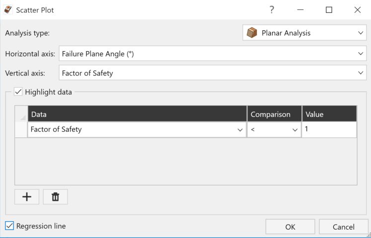
- Click OK to generate the scatter plot.
A scatter plot of the Failure Plane Angle (°) vs. the Factor of Safety for Planar Analysis is displayed in the Scatter Plot View.
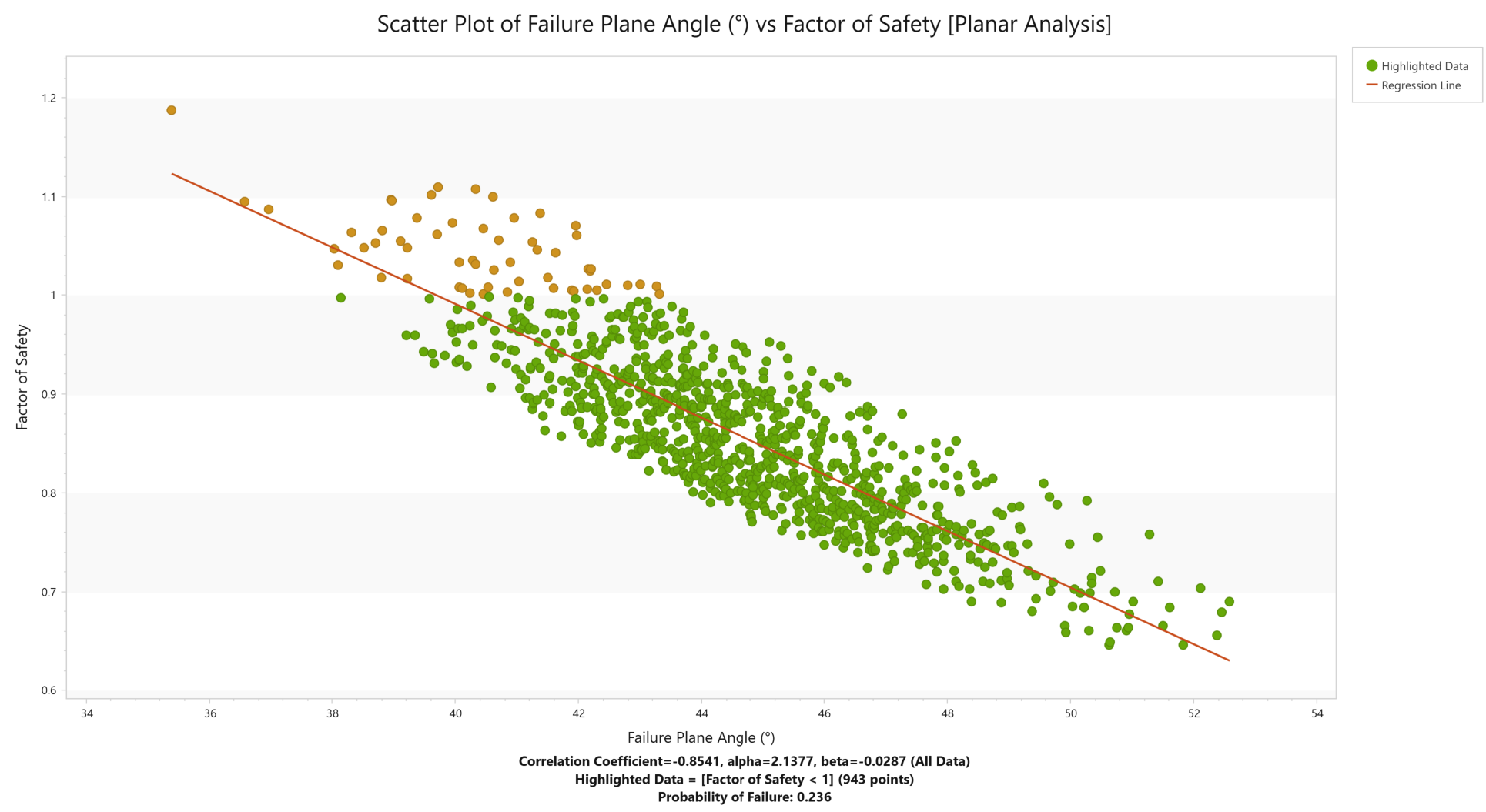
There appears to be relatively good correlation between Factor of Safety and Slope Dip. From the highlighted (failed) block data, it can be readily seen that block failures correspond to relatively steeper Slope Dip, as we would expect.
The alpha and beta values of the regression line are shown at the bottom of the plot.
Note the following:
- The alpha value (2.1377) represents the y-intercept of the linear regression line on the scatter plot.
- The beta value (-0.0287) represents the slope of the linear regression line.
- The Correlation Coefficient (-0.8541) indicates the degree of correlation between the two variables plotted. This value varies between -1 and 1, where a number close to 0 indicates a poor correlation, and a number close to 1 or -1 indicates a good correlation. A negative Correlation Coefficient indicates the slope of the regression line is negative.
You can plot scatters of various input and output variable pairs (i.e. wedge information, forces, stresses, slope geometry, etc.). The scatter plot data can be easily changed without leaving the Scatter Plot View using Change Plot Data option, as discussed in Histogram Plots.
5.3.1 Picked Block (Viewing Other Blocks)
Now tile the Scatter Plot View and the 3D Planar View so that both are visible.
- Select Home > Window > Tile Vertically

- Select Planar Analysis on the analysis toolbar to maximize the 3D Planar View.
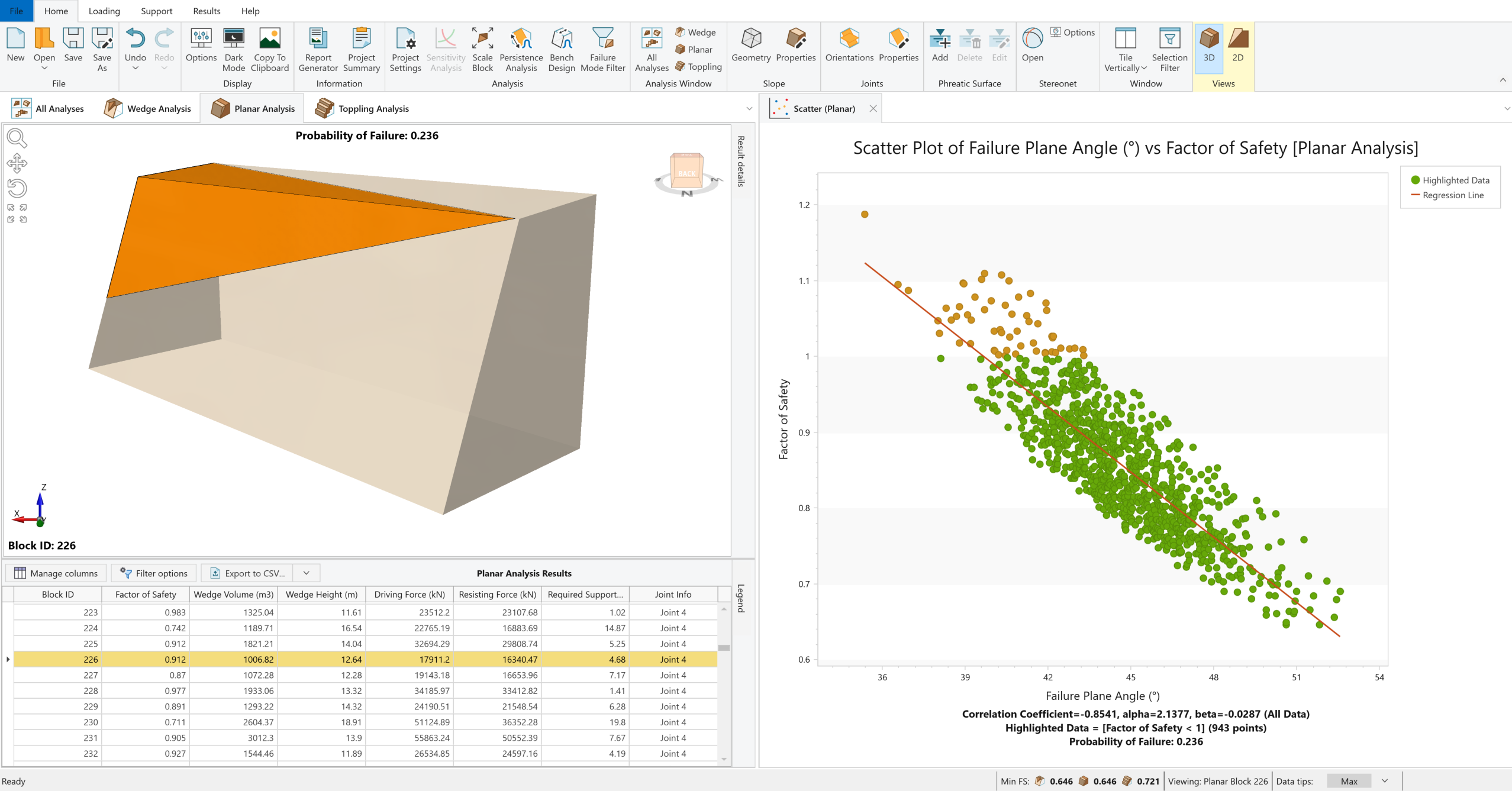
A useful feature of Scatter plots is the ability to view other blocks. Double-clicking on the plot displays the nearest corresponding block in the corresponding 3D View.
Double-click at any point along the scatter and notice that a different block is now displayed in the 3D Planar View. Also notice that the Factor of Safety and details of this picked block are now displayed in the Results Grid. Double-click on various points along the Scatter and notice different blocks are displayed in 3D Planar View as well as the corresponding Factor of Safety values are displayed in Results Grid.
This feature is applicable for all analysis methods (wedge, planar and toppling) and allows you to view any block generated by the Probabilistic analysis corresponding to any point along the scatter distribution.
Close the Scatter Plot by clicking the X on the Scatter Plot tab or Close icon on the toolbar.
5.4 Cumulative Distributions (S-Curves)
In addition to histograms and scatters, you can also plot Cumulative Distributions (S-curves) of the statistical results (i.e., Cumulative plots), using the Cumulative Plot option.
- Select Results > Charts > Cumulative
 on the toolbar.
 - In the Cumulative Plot dialog, set Analysis Type = Planar Analysis.
- Set Data to Plot = Factor of Safety.
- Set Number of Bins = 60.
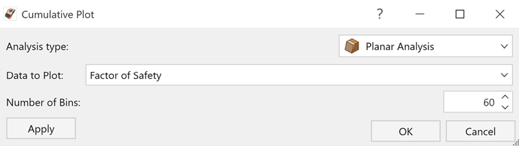
- Click OK to generate the cumulative plot.
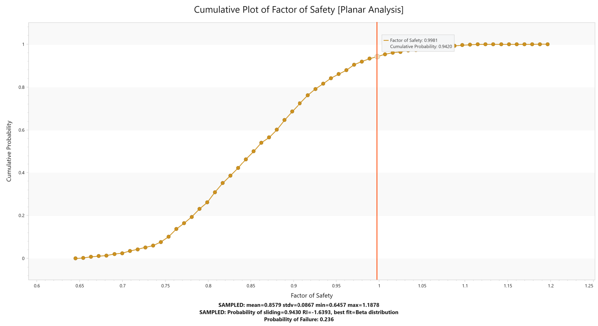
A cumulative Factor of Safety distribution for Planar Analysis is generated, as shown below.

A point on a cumulative probability curve gives the probability that the plotted variable is less than or equal to the value of the variable at that point.
For a cumulative Safety Factor distribution, the cumulative probability at Safety Factor = 1 is equal to the Probability of Sliding. We can demonstrate this on the Cumulative Plot.
- Move your cursor on the Cumulative Plot. You'll see a crosshair vertical line that follows the cursor.
- Move the cursor anywhere over the cumulative probability curve to see a popup data tip that shows the Factor of Safety and Cumulative Probability at that point on the curve.
- Move the cursor until you approximately see Safety Factor = 1.
Notice that the Cumulative Probability = 0.9420 when FS=0.9981, which is almost equal to the Probability of Sliding for Planar Analysis for this example, as shown in the figure below.
Close the Cumulative Plot by clicking the X on the Cumulative Plot tab or Close icon on the toolbar.
5.5 Constant vs. Variable Pseudo-Random Sampling
In RocSlope2, Constant Pseudo-Random sampling is in effect for a Probabilistic analysis by default. So far in this tutorial we have used the default Constant Pseudo-Random sampling option, set in the Statistics tab of the Project Settings dialog (see Section 4.1.3 of this tutorial).
Constant Pseudo-Random sampling allows you to obtain reproducible results from a Probabilistic analysis by using the same seed value to generate random numbers. This results in identical sampling of the input data distributions each time the analysis is run (with the same input parameters). The Probability of Failure, Mean Safety Factor, and all other analysis output are reproducible. This is why you can obtain the exact values shown in this tutorial. This can be useful for demonstration purposes or to discuss example problems.
We will now demonstrate how different outcomes can result from a Probabilistic analysis by allowing a variable seed value to generate the random input data samples.
You can change the sampling option to Variable Pseudo-Random using the Project Settings dialog. The Variable Pseudo-Random option uses a different seed number each time you re-compute, resulting in a different sampling of your input data distributions and therefore different analysis results.
- Select Home > Analysis > Project Settings on the toolbar.
- Navigate to Statistics
 tab.
tab. - Under Pseudo-Random Number Generation, select Variable Seed Based on Time .
- Click OK.
As discussed earlier in this tutorial, to ensure the latest analysis results are always displayed, RocSlope2 automatically computes an analysis whenever input data is entered or modified in a dialog and Apply or OK is clicked. Notice that the Probability of Failure (PoF) for Wedge, Planar and Toppling analyses are computed instantly considering new random seed number resulting in a different sampling of your input data distributions, and consequently different analysis results.
Now re-select the Project Settings again and click OK. Notice that after each re-compute:
- The Results Grid is updated and displays new results.
- The Probability of Failure is, in general, different each time the analysis is run.
This demonstrates the difference between Constant and Variable Pseudo-Random sampling.
- Now change the Pseudo-Random sampling back to Constant in Project Settings.
5.6 Sampling Method
So far, we have used Latin Hypercube sampling throughout this tutorial. As an additional exercise, let’s try Monte Carlo sampling, with a smaller number of samples. You change this in the Project Settings dialog.
- Select Home > Analysis > Project Settings
- Navigate to Statistics tab.
- Set Sampling Method = Monte-Carlo
- Set Number of Samples = 500
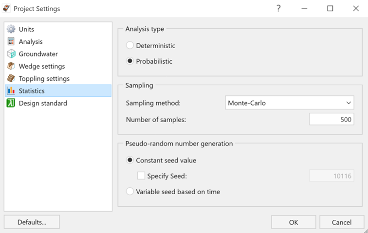
- Click OK to apply the changes and close the dialog.
Analyses will re-compute instantly. Examine the Probability of Failures and the Factor of Safety Histograms for each analysis method. The results should be similar to the Latin Hypercube analysis.
The difference, as shown in the figures below for Failure Plane Angle (°) Histogram for Planar Analysis, is in the sampling of the input data random variables. Notice that the Monte Carlo sampling method results in a much more variable sampling of the input data distribution compared to the Latin Hypercube method, which gives smoother results.
6.0 Failure Mode Filter
We will now look at the ability in RocSlope2 to filter wedges by failure mode in Wedge Analysis.
- Select Home > Analysis > Failure Mode Filter

- Select the Apply Failure Mode Filter check box to activate the filter options. By default, all filters are selected.
- De-select Allow sliding on both joint 1 and joint 2.
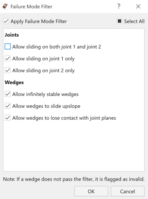
- Click OK to apply the filters.
Wedge Analysis will re-compute instantly. Wedges sliding along on both Joint 1 and Joint 2 will be filtered and they will be flagged as invalid.
This means that all the wedges generated in this Wedge Probabilistic analysis will fail by sliding along either Joint 1 or Joint 2 only.
Examine the blocks in Results Grid and check Result Details in 3D Wedge View for a more detailed summary of each wedge.
- Re-select Failure Mode Filter on the toolbar.
- De-select the Apply Failure Mode Filter checkbox to deactivate filtering options.
- Click OK to apply changes.
7.0 Export Data
RocSlope2 has the following options in the Results Grid for exporting results:
- Export current results to CSV
- Export current results to Excel
- Export all results to CSV
- Export all results to Excel
To export the currently viewed slope and result block geometry as an .obj file select File > Export 3D Geometry  Finally, after generating any graph in RocSlope2, you can easily export the data to Microsoft Excel as follows:
- Select the Chart in Excel button on the toolbar or right-click on a graph and select Plot in Excel from the popup menu.
- Export the graph data and generate a graph in Excel.
8.0 Additional Exercise
8.1 Correlation Coefficient for Cohesion and Friction Angle
In this tutorial, Cohesion and Friction Angle were treated as completely independent variables. In fact, it is known that Cohesion and Friction Angle are related in a general way, such that materials with low friction angles tend to have high cohesion, and materials with low cohesion tend to have high friction angles.
You can use the Define Joint Properties dialog to define the degree of correlation between Cohesion and Friction Angle for Joint Strength Properties. This only applies if:
- BOTH Cohesion and Friction Angle are defined as random variables (i.e., assigned a Statistical Distribution), and
- Statistical Distribution = Normal/Uniform/Lognormal/Exponential/Gamma (will not work for Beta or Triangular).
As a suggested exercise, try the following:
- Select Home > Joints > Properties to open the Joint Properties dialog.
- Select Joint Property 2.
- Notice that BOTH Cohesion and Friction Angle are assigned Lognormal Statistical Distribution.
- Select the Correlate Cohesion and Phi checkbox.
- Ensure that Correlation Coefficient = -0.5 (initially, use the default value of –0.5).

- Click OK and re-run the analysis.
- Now repeat steps 1 to 6, using Correlation Coefficients of -0.6 to -1.0, in 0.1 increments and re-examine the analysis results.
When the probabilistic analysis is run, the sampling of the random variables will be correlated according to your input.
In general, this should provide more realistic analysis results, compared to running the analysis with no correlation of variables.
This concludes the tutorial. You are now ready to proceed to the next tutorial, Tutorial 6 – Persistence Analysis & Bench Design.