6 - Persistence Analysis & Bench Design
1.0 Introduction
In this tutorial, we will explore the probabilistic analysis of a slope, focusing on the distribution of joint persistence, the spatial variation in their locations, and the design features of the bench.
Topics Covered in this Tutorial:
- Persistence Analysis
- Bench Design
Finished Product:
The finished product of this tutorial, Bench_And_Persistence_Analysis_Final.rocslope2, can be found in the Examples > Tutorials > Tutorial 6 folder within your RocSlope2 installation directory.
2.0 Starter File
When the program starts, a default model is automatically created. To load the starter file:
- Select File > Open Project and navigate to the Examples > Tutorials > Tutorial 6 folder in your RocSlope2 installation directory.
- Open the Bench_And_Persistence_Analysis_Starter.rocslope2 file.
2.1 Project Settings
In this tutorial, units are set to Metric, stress as kPa. The settings are configured to perform Probabilistic Analysis with Monte Carlo as the Sampling Method for 500 samples across all three failure modes: Wedge, Planar, and Toppling.
2.2 Slope Geometry
Slope Geometry is the input data dialog for entering slope geometry data in RocSlope2.
- Select Home > Slope > Geometry

- The following data is included in the starter file:
Slope Face |
Statistics Defined |
|
Slope Face Dip (°) |
70 | Yes |
Slope Face Dip Direction (°) |
45 | No |
Height (m) |
20 | No |
Overhanging |
No | - |
Use Default length |
No | - |
Length (m) |
50 | No |
Upper Face |
||
Dip (°) |
5 | Yes |
Dip Direction (°) |
45 | No |
Use Default Bench Width |
No | - |
Bench Width (m) |
10 | No |
Overall Base Inclination (for Toppling) |
||
Overall Base Inclination / Dip (°) |
42 | No |
Tension Crack Exists |
No | - |
As we can notice, statistics are only defined for Slope Face Dip and Upper Face Dip with following parameters:
- Slope Face Dip: Distribution is Normal, Mean is 70, Standard Deviation is 3 with Relative Minimum and Maximum as 9 and 9 respectively.
- Upper Face Dip: Distribution is Triangular, Mean is 5 with Relative Minimum and Maximum as 2 and 2 respectively.
2.3 Slope Properties
The Slope Properties dialog is used for entering the data for Rock Unit Weight, Water Parameters and Rock Material Strength if Block Flexure Toppling is enabled.
- Select Home > Slope > Properties
 . The following data is expected:
- Material Strength
- No statistics defined, Unit Weight (kN/m3) = 26
- Water Parameters
- Apply Ponded Water = No
- Groundwater Method = Dry
2.4 Joint Properties
The Joint Properties dialog is used to define the Joint Strength (Strength Type and Parameters) and Water Parameters (Pressure Distribution Model and data).
- Select Home > Joints > Properties

- The following Joint Property data is shown:
| Strength | |||||||
| Joint Property | Strength Type | Cohesion (kPa) | Phi (°) | Tensile Strength (kPa) | Correlate Cohesion and Phi | Correlation Coefficient | Waviness (°) |
| 1 | Mohr-Coulomb | 0 | 40 | 0 | No | - | 0 |
| 2 | Mohr-Coulomb | 5 | 32 | 0 | Yes | -1 | 2 |
- Joint Property 1:
- Phi: Distribution is Lognormal, Mean is 40, Standard Deviation is 2 with Relative Minimum and Maximum as 2 and 4 respectively.
- Joint Property 2:
- Cohesion: Distribution is Lognormal, Mean is 5, Standard Deviation is 1 with Relative Minimum and Maximum as 2 and 3 respectively.
- Phi: Distribution is Lognormal, Mean is 32, Standard Deviation is 2 with Relative Minimum and Maximum as 2 and 6 respectively.
- Click OK to close the dialog.
2.5 Joint Orientations
The Joint Orientations dialog is used to define the Joint Orientations (Dip, Dip Direction), assign a Joint Property to each joint, define Joint Spacing for toppling analysis, and set Lateral Limits for sliding and toppling joints if desired.
- Select Home > Joints > Orientations

- Sliding Joint Later Limits (°) should be 20.
- Under Toppling Analysis Settings, Joint Spacing should be 2 m.
- Toppling Joint Later Limit (°) should be 30.
- Base Joint Property should be set to Joint Property 2.
- For Statistics Settings, Orientation Definition Method is Fisher and Fisher Options is Standard Deviation.
- Input data for Joint Orientation is as follows:
| Joint No | Mean Dip (°) | Mean Dip Direction (°) | Std. Dev. | Joint Property |
| 1 | 70 | 14 | 0 | Joint Property 1 |
| 2 | 65 | 220 | 7 | Joint Property 1 |
| 3 | 74 | 145 | 0 | Joint Property 1 |
| 4 | 45 | 52 | 4 | Joint Property 1 |
3.0 Persistence Analysis
In standard Wedge and Planar analysis, the program determines the maximum wedge size by automatically scaling a wedge to fit the slope dimensions. This conservative approach affects the Probability of Failure in a Probabilistic Analysis. Often, the spatial location and persistence of joints limit the formation of valid wedges. For a slope with specific Length, Height, and Bench Width, only certain joint plane locations result in valid wedges. Similarly, a wedge does not form if the joint Persistence is below a certain threshold.
In Persistence Analysis, statistical distribution for Joint Persistence or Joint Trace Length is used to scale the wedge size, and the program generates a wedge if possible. This refines the calculation of the Probability of Failure. RocSlope2 incorporates these factors in the Probabilistic analysis.
3.1 Joint Spacing Types
There are two different Joint Spacing options available for a Persistence analysis:
- Large Joint Spacing: It is assumed there is only one trace of Joint 1 and one trace of Joint 2 on the slope face. It is lower bound solution for probability of failure.
- Small Joint Spacing (Ubiquitous Joints): It is assumed that there is spacing (repeated joints) associated with the two joint sets Joint 1 and Joint 2. There is no longer one wedge but several possible wedges that can form on the slope. It is an upper bound solution for Probability of Failure.
Small Joint Spacing model automatically scales down the wedge size until the persistence conditions are met. So, a wedge is almost always formed in each simulation if the geometry of the joints and slope creates a kinematically feasible wedge.
For more information, see Persistence Analysis.
3.2 Performing Persistence Analysis
To add Persistence Analysis:
- Select Home > Analysis > Persistence Analysis

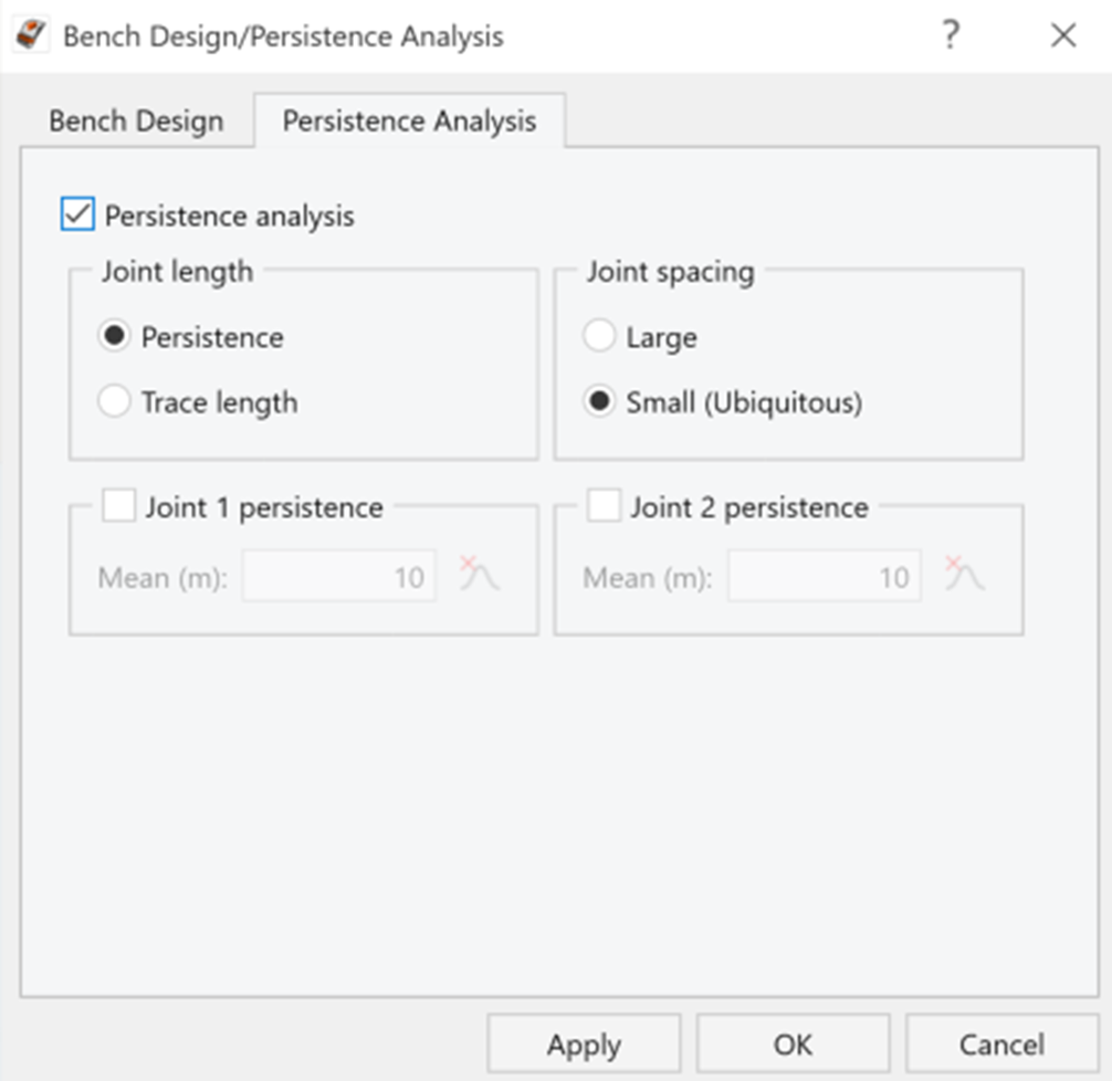
- The Bench Design/ Persistence Analysis dialog appears.
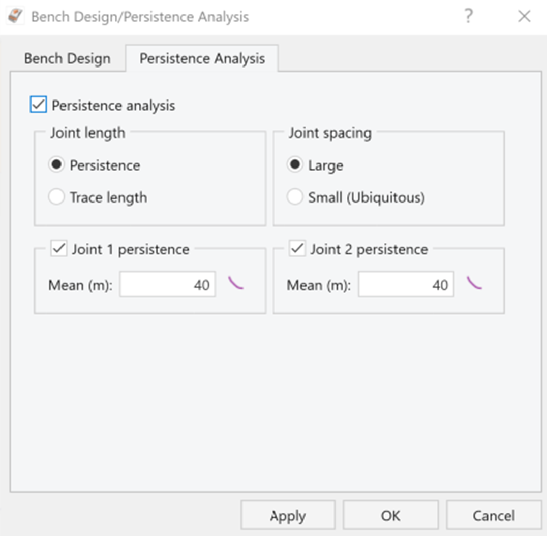
- Under the Persistence Analysis tab, select the Persistence Analysis checkbox.
- For Joint Length we will select Persistence, and for Joint Spacing we will select Large.
- We will also define statistics for Joint 1 and Joint 2 persistence. Please select both and define following data:
- Joint 1 persistence: Distribution is Exponential, Mean is 40, with Relative Minimum and Maximum as 20 and 40 respectively.
- Joint 2 persistence: Distribution is Exponential, Mean is 40, with Relative Minimum and Maximum as 20 and 40 respectively.
- Click OK.
3.3 Persistence Analysis Results
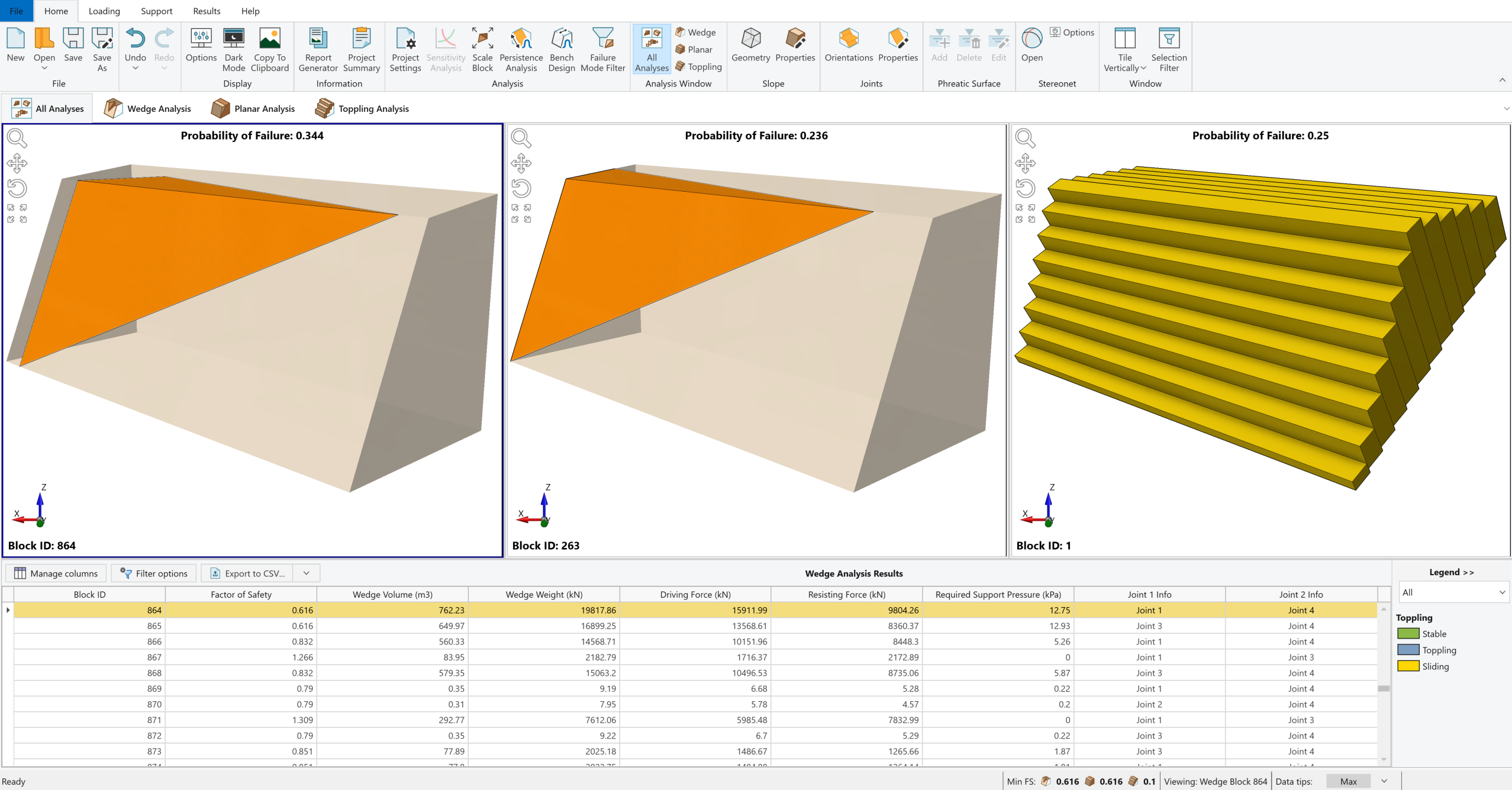
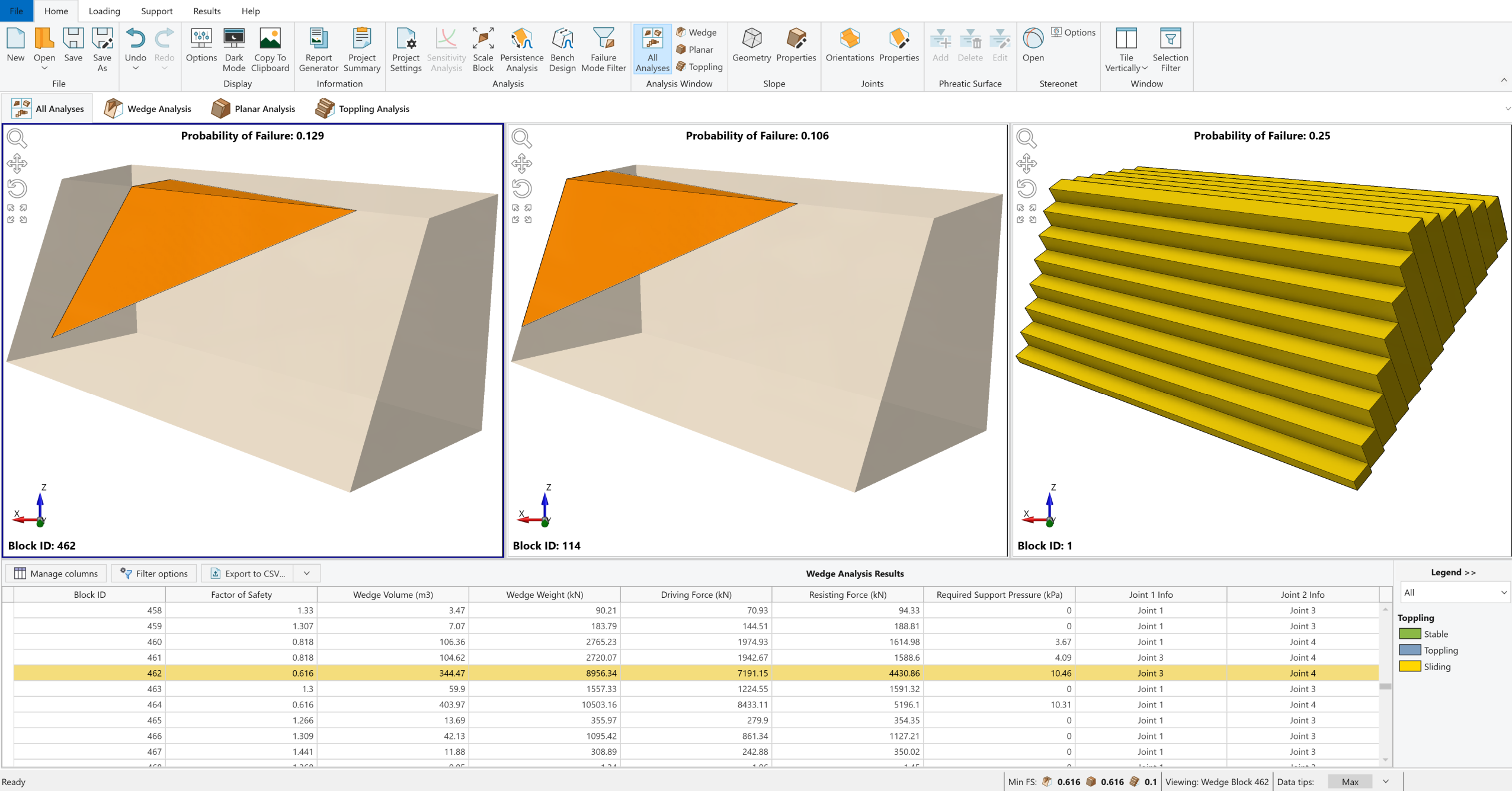
Computation of 500 Monte Carlo samples occur, and the Probability of Failure is calculated. For every one of the 500 simulations, a value of Joint Persistence is sampled. Because the Large Joint Spacing option is selected, if the wedge that is formed based on the random location of the joint planes has Joint Persistence values that exceed the sampled values, the wedge is flagged as invalid.
The figure below illustrates the results of the computation.
3.4 Histogram Plots of Results
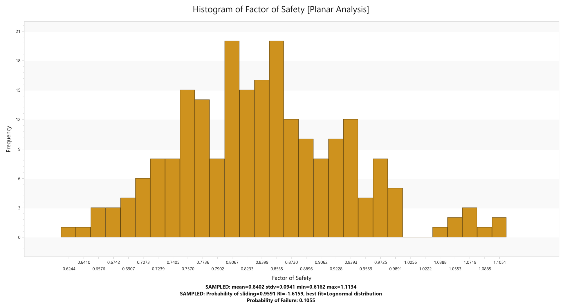
Several useful features exist for the display of data from a Probabilistic Analysis. For example, to get an idea of the relative distribution of failed to stable samples, we can plot a histogram of the Factor of Safety. To open the Histogram Plot Parameters dialog:
- Select Results > Charts > Histogram

- Enter the following:
- Analysis Type = Planar Analysis
- Data to Plot = Factor of Safety
- Number of Bins = 30
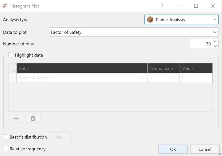
Histogram Plot dialog - Click OK.
A Factor of Safety histogram is displayed.
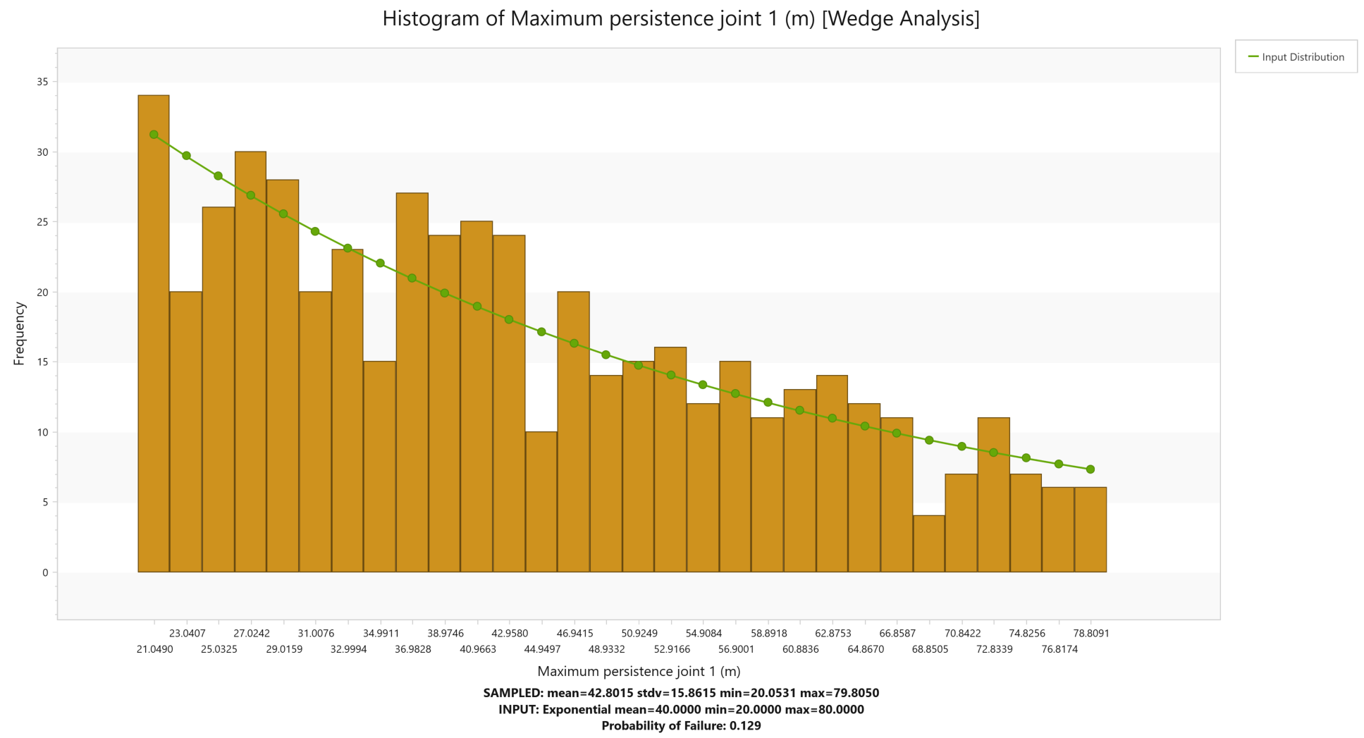
Now let’s plot the maximum Persistence of Joint 1 for Wedge Analysis that was statistically generated as part of the Persistence analysis.
- Select Results > Charts > Histogram
- Enter the following:
- Analysis Type = Wedge Analysis
- Data to Plot = Maximum Persistence Joint1
- Number of Bins = 30.
- Select the Input Distribution check box.
- Click OK to generate the histogram.
Similarly, a histogram can be created for Maximum Persistence of Joint 1 in Planar Analysis.
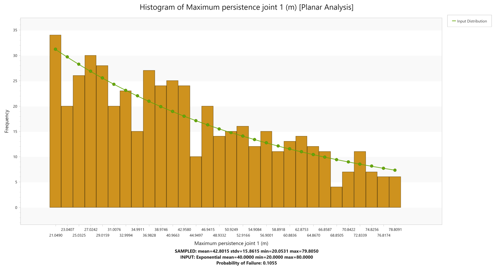
Remember that we defined an exponential distribution of Joint Persistence 1 that varied between 20 m and 80 m with a mean of 40 m. Note that the histogram does not match this input distribution (the green line) evenly. This is because we are using the Monte Carlo method of sampling. If we use Latin HyperCube as our sampling method, we will be able to get more even sampling with a smaller data size.
4.0 Bench Design
Slope instabilities in open pit mine present a significant design challenge in geotechnical engineering. Such failures can be controlled by major structures such as faults or lithologic contacts, which have sufficient lengths to affect overall stability, or by more numerous, smaller structures such as joints, foliations, and bedding planes. Only analyzing potential large-scale slope failures may result in unanticipated instabilities caused by Bench Failure. Hence, it is crucial to establish and maintain adequate bench width to catch and control the structural failures, ensuring safe and reliable access to the slopes for continuous engineering operations.
The Bench Design option in RocSlope2 helps analyze bench-scale failures, which can directly influence the overall slope angle and must therefore be considered. This option extends the Probabilistic analysis features in RocSlope2 for Wedge and Planar Analyses. By assuming either a constant bench width or constant inter-ramp angle, you can input design parameters and statistical information to optimize the Bench Design according to design constraints and field measurements.
In RocSlope2, two design approaches are available to assess the stability of bench-scale wedges for a range of bench face angles:
- Managed Approach to Slope Design: The user can assess the number of failed wedges and minimum bench width required for each bench face angle.
- Quantitative Hazard Assessment: The user can estimate the likelihood of forming different wedge sizes (Probability of Occurrence) and the likelihood that such wedges will slide (Probability of Sliding), which provides an estimate of the Probability of Failure for various back-break distances.
Both approaches provide valuable information on bench loss and assist the user in selecting an optimum bench face angle.
For more information, see Bench Design.
4.1 Performing Bench Design
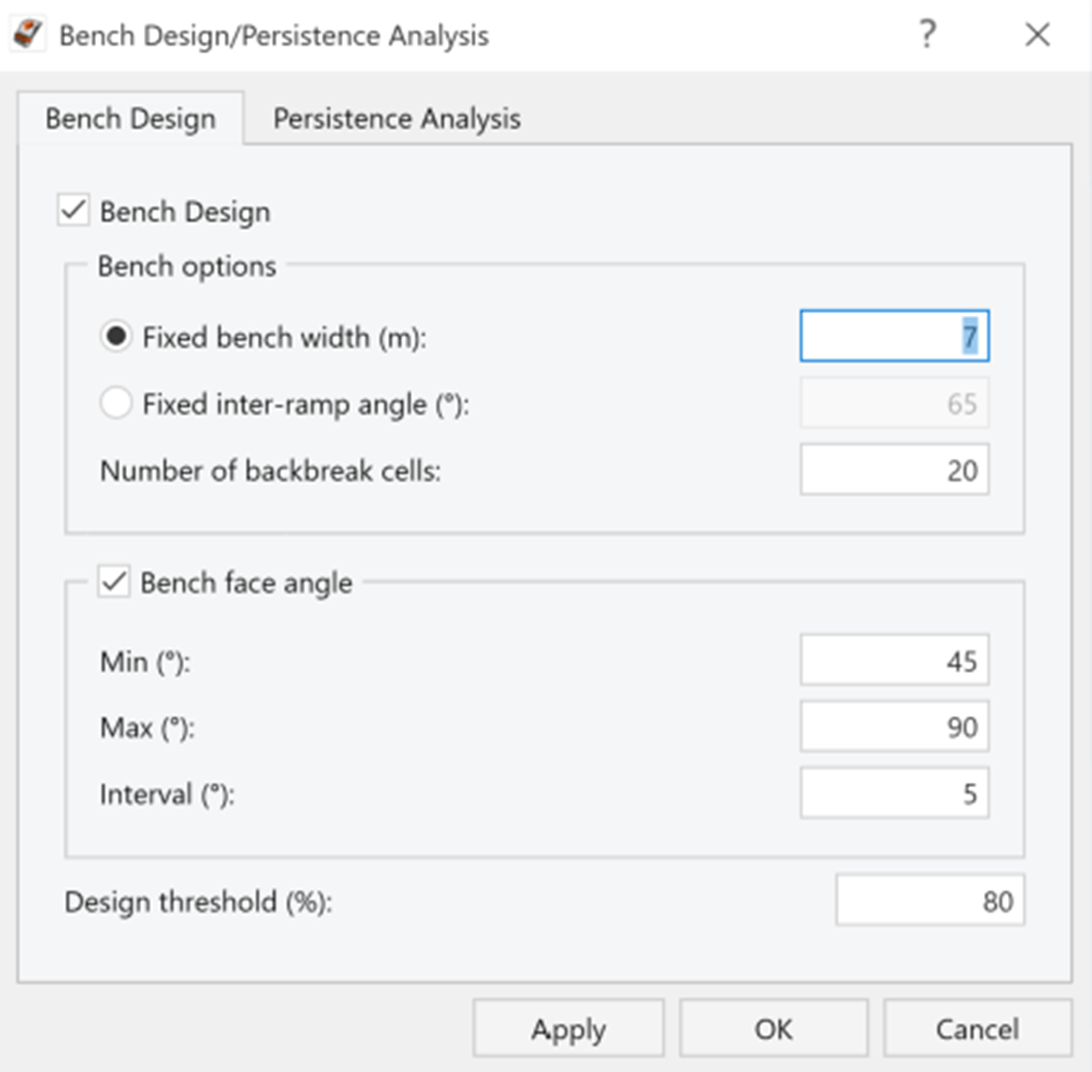
- Select Home > Analysis > Bench Design

- The Bench Design/ Persistence Analysis dialog appears. Under the Bench Design tab, select the Bench Design checkbox.
- In this tutorial we will perform a Fixed Bench Width analysis. Select Fixed Bench Width and enter 7 m.
- Select the Bench Face Angle check box and make sure that its values are Min (º) = 45, Max (º) = 90 and Interval (º) = 5.
Bench Analysis Inputs - Under the Persistence Analysis tab, set Joint Spacing as Small (Ubiquitous)
and deselect Joint Persistence 1 and Joint Persistence 2. Here we will assume infinite persistence.
Persistence Analysis Inputs - Click OK.
4.2 Bench Design Results
Computation of 500 Monte Carlo samples occur for each bench face angle (45, 50, 55, 60, 65, 70, 75, 80, 85, 90 degrees in this case). During this assessment, each valid wedge is assigned to one of the backbreak cells based on the width of the wedge measured from the crest. As an example, if a wedge has a width from the crest of 0.4m, it is assigned to the 0.35-0.7m backbreak cell.
As mentioned earlier, two approaches are available to interpret the data from the bench analysis, managed approach to bench design and a quantitative hazard analysis. Now we will look at each of these.
4.2.1 Managed Approach
In open-pit mining, it is often acceptable to use steeper bench face angles and allow some failures to occur if safety is not compromised. While this will result in a greater amount of failed material on the bench (this is referred to as the spill width), the cost of regular bench cleanups is significantly less than the cost of excavating additional waste rock when using shallow bench angles. This concept, referred to as a managed approach, can be utilized in RocSlope2 through various plots.
To create Total Probability of Failure Plot:
- Select Results > Charts > Bench Design
- The Bench Design Chart Options dialog appears. Select Analysis Type = Wedge and Chart Type = Total Probability of Failure.
- Click OK.
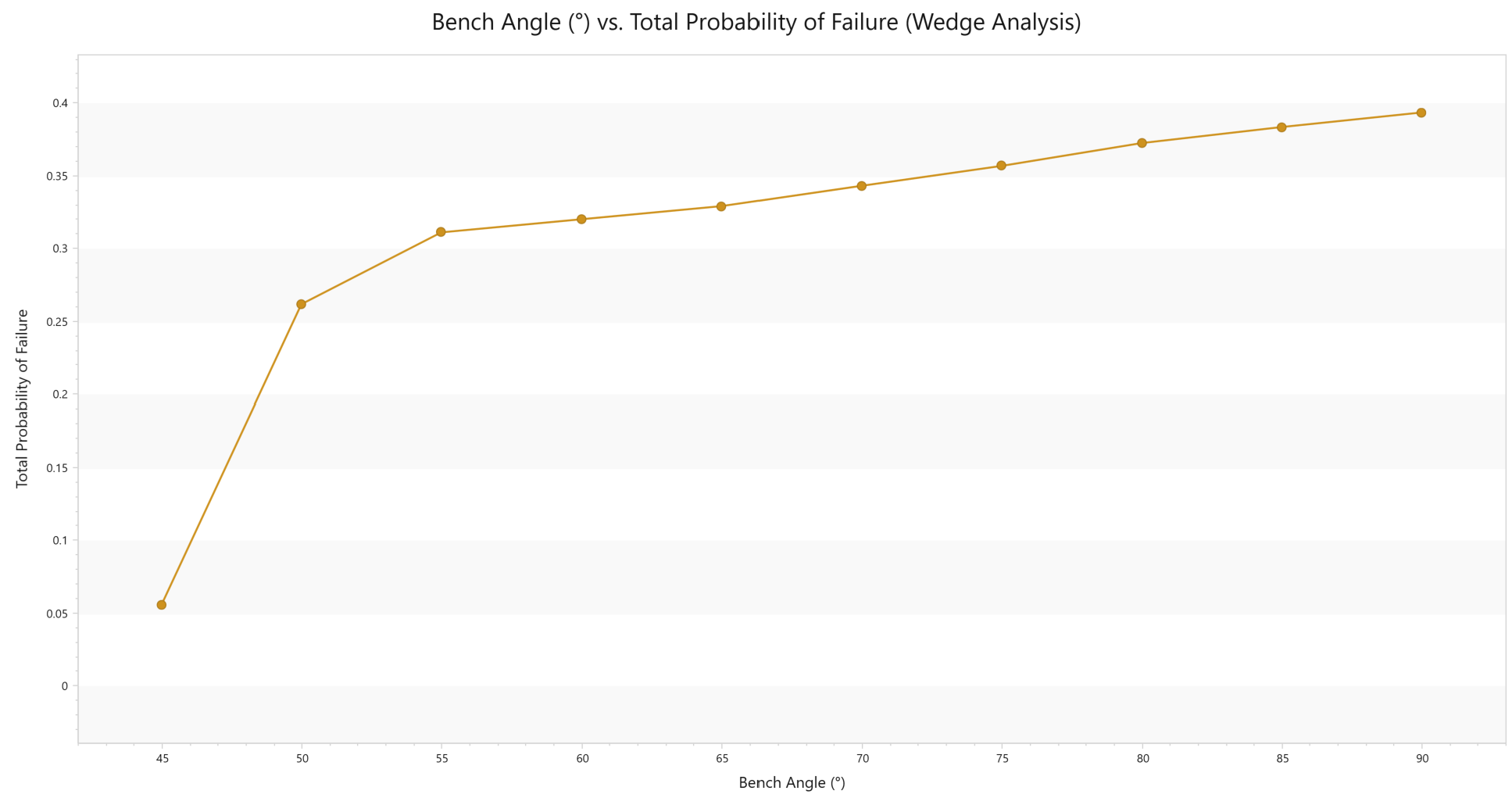
This shows that the Total Probability of Failure (and therefore the number of failed wedges) increases as the bench face angle increases from 45º to 90º. This is logical as one would expect more failed wedges for a steeper slope.
Similarly, the graph can be created for Planar Analysis as well.
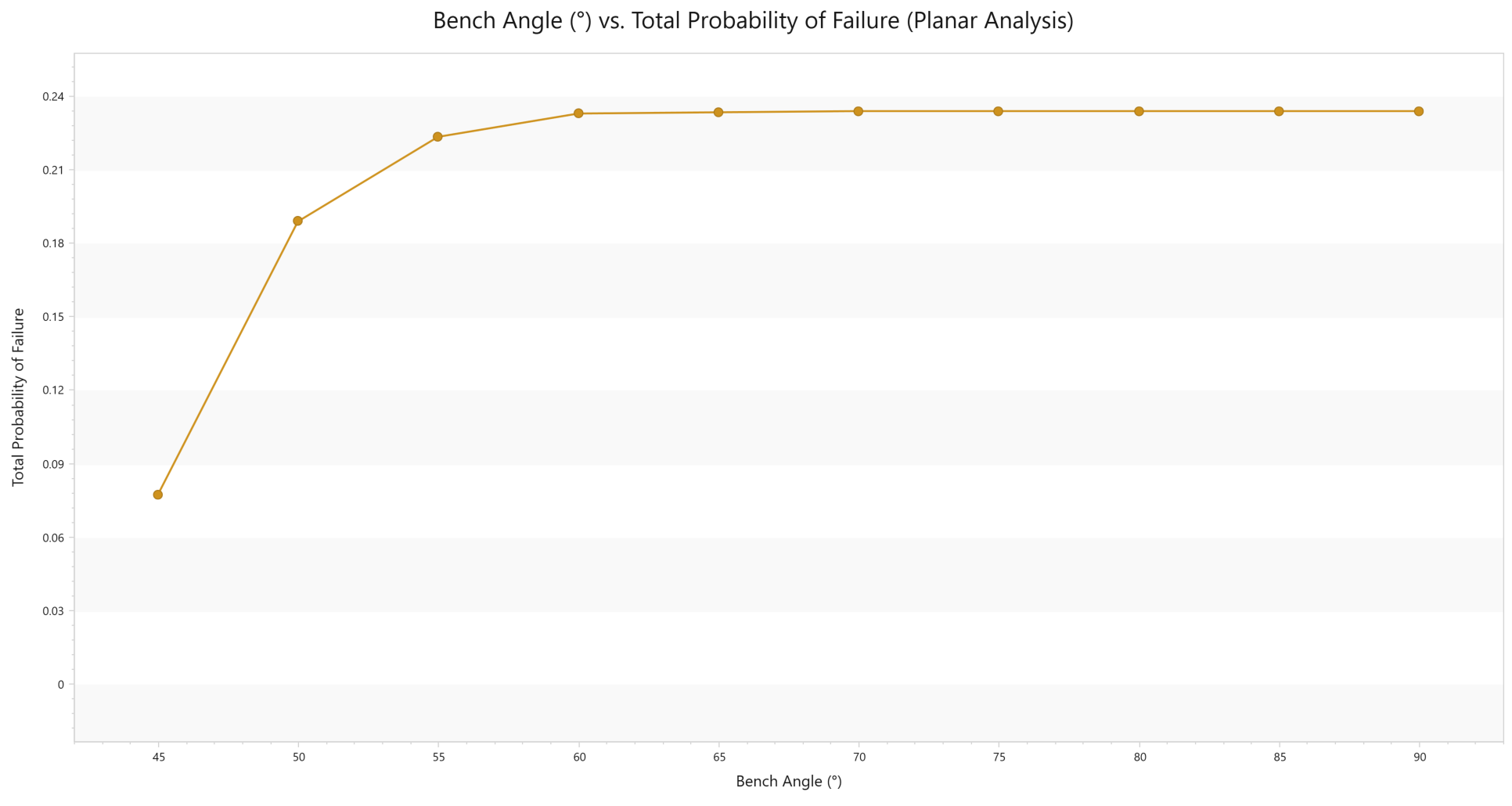
This shows that the Total Probability of Failure is consistent as the bench angle increases from 45º to 90º for Planar Analysis.
4.2.2 Quantitative Hazard Analysis
While the managed approach can be used to determine the number of failed wedges for each bench face angle, it does not provide information on the expected wedge size and amount of bench loss. To determine this, a Quantitative Hazard Assessment (QHA) is needed. A QHA calculates the probability that the bench will fail to a certain backbreak distance. Such an analysis is useful on its own but can also be combined with an estimate of the potential cost of bench loss to calculate the expected risk.
To interpret the output of the QHA, some terms must first be defined:
- Cell Probability of Occurrence: For a given backbreak cell, this is the number of valid wedges in the cell divided by the total number of blocks generated.
- Cell Probability of Sliding: For a given backbreak cell, this is the number of valid wedges with a factor of safety less than 1.0 (failed) divided by the number of valid wedges.
- Cell Probability of Failure: For a given backbreak cell, this is the Probability of Occurrence for the cell multiplied by the Probability of Sliding for the cell.
When dealing with a QHA, information on joint persistence should be used. In this way, the location and size of the wedge is better determined.
First, close all graph views.
We will update the Persistence Analysis data as follows:
- Select Home > Analysis > Persistence Analysis
- The Bench Design/ Persistence Analysis dialog appears. For Joint Length, we will select Persistence and for Joint Spacing we will select Small.
- We will also define statistics for Joint 1 and Joint 2 persistence. Please select both and define following data:
- Joint 1 persistence: Distribution is Exponential, Mean is 25, with Relative Minimum and Maximum as 5 and 10 respectively.
- Joint 2 persistence: Distribution is Exponential, Mean is 25, with Relative Minimum and Maximum as 5 and 10 respectively.
- Click OK.
To create the Cell Probability of Occurrence Plot:
- Navigate to Results > Charts > Bench Design
- The Bench Design Chart Options dialog will appear. Select the Analysis Type as Wedge and Chart Type as Cell Probability of Occurrence.
- Click OK.
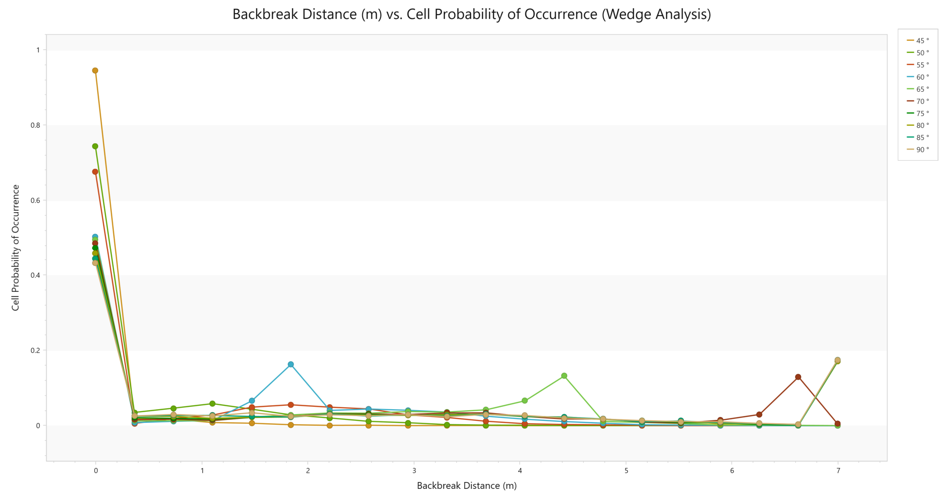
This plot shows that the most likely backbreak distance (represented by the peak of the curve) for; 45°, 50° and 55° is 0.0m, 60° is 1.8m, 65° is 4.4m, 70° is 6.6m and 75°, 80°, 85° and 90° is 7.0m. Larger wedges are also seen to be more common for steeper bench face angles, given the longer “tails” in the curve. This is more clearly demonstrated through a Cell Cumulative Probability of Occurrence plot.
- Select Change Plot Data and plot the Cell Cumulative Probability of Occurrence Plot for the Wedge Analysis:
Now that the likelihood of different wedge sizes is better understood, the probability that a wedge with a given backbreak distance will slide (factor of safety < 1.0) can be examined.
- Select Change Plot Data and plot the cell Probability of Sliding for the Wedge Analysis:
This plot shows that for shallow bench face angles (45 to 60deg) smaller wedges (which have smaller backbreak distances) have the greatest Probability of Sliding. For steeper bench face angles (65 to 90deg), the probability of sliding is seen to decrease initially, then increases to their maximum value between 3-4m backbreak distance before a consistent minimum value is obtained. This indicates that for steeper bench face angles, larger wedges are a more significant concern when considering bench loss.
By multiplying the Probability of Occurrence and Probability of Sliding for each cell, a Probability of Failure for the cell can then be obtained. This helps to identify the backbreak distances that are most likely to fail when designing the open pit for each bench face angle. When multiplied by the Consequence of such a failure (typically represented as a cost), the risk for the slope can be assessed.
This concludes the tutorial.