2 - Synthetic Joint Set
1.0 Introduction
Joint sets are groups of joints which have similar orientations. Using distributions of joint set orientation, spacing, and size, we can statistically sample and generate joints across a provided traverse (i.e., scanline, borehole, etc.). This tutorial covers the use of synthetic joints in RocTunnel3.
Finished Product
The finished product of this tutorial can be found in the Synthetic Joint Set.roctunnelmodel file. All tutorial files installed with RocTunnel3 can be accessed by selecting File > Recent Folders > Tutorials Folder from the RocTunnel3 main menu.
2.0 Opening the Starting File
- Select File > Recent > Tutorials Folder in the menu.
- Go to the Synthetic Joint Sets folder and open the starting file Synthetic Joints Sets - starting file.roctunnelmodel.
This model already has the following defined and provides a good starting point to start defining synthetic joint sets:
- Project Settings
- Material Properties
- External Geometry
- Joint Properties
2.1 Project Settings
Review the Project Settings.
- Select Analysis > Project Settings or click on the Project Settings
 icon in the toolbar.
 - Select the Units tab. Ensure Units are Metric, stress as MPa
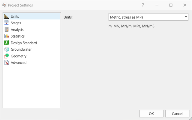
Units Tab in Project Settings dialog - Select the Analysis tab.
- Ensure Design Factor of Safety = 1.2.
- Ensure Successive Failure = OFF. We will only be analyzing the blocks which are exposed on the excavation and are readily removable.
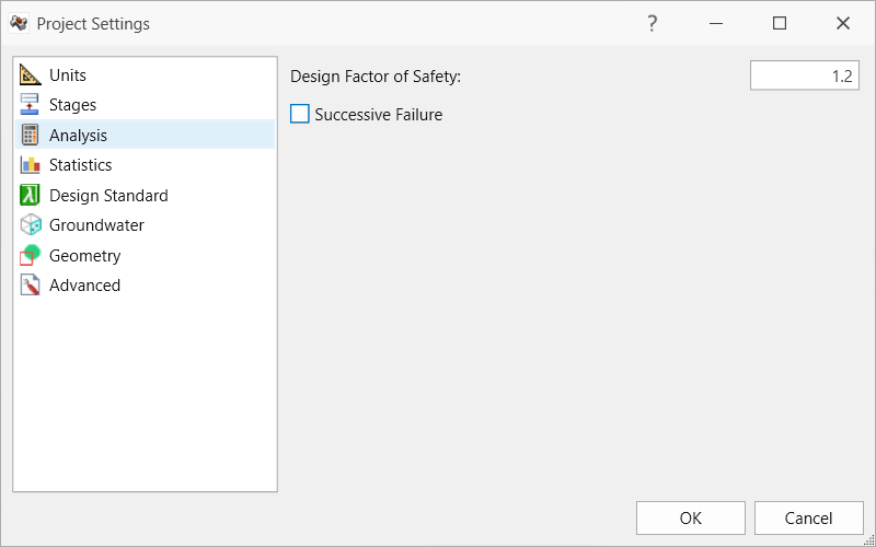
Analysis Tab in Project Settings dialog - Select the Statistics tab.
- Ensure Synthetic Joint Sampling = Latin Hypercube and keep everything else as default.
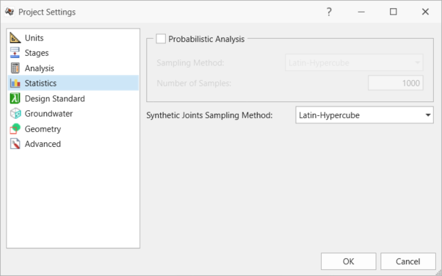
Statistics tab in Project Settings dialog - Click Cancel to exit the dialog.
2.2 Material Properties
Review the Material Properties.
- Select Materials > Define Materials in the menu or click the Define Materials
 icon in the toolbar.
 - In the Define Materials dialog, two (2) material properties are defined.
- The Zone I material property has:
- Unit Weight = 0.026 MN/m3
- No Water Surface applied.
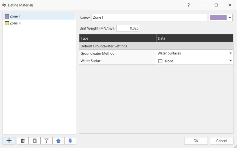
Zone I Material Property in Define Materials dialog - The Zone II material property has:
- Unit Weight = 0.025 MN/m3
- No Water Surface applied.
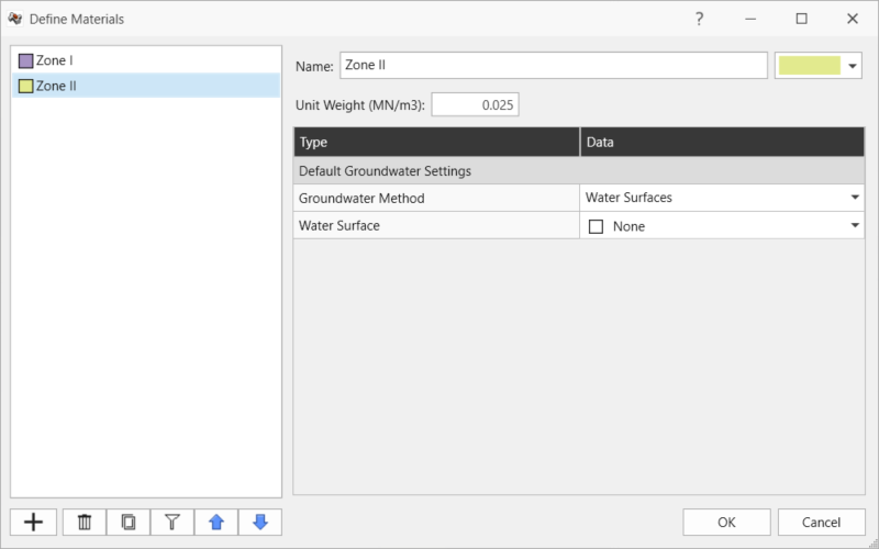
Zone II Material Property in Define Materials dialog - Click Cancel to exit the dialog.
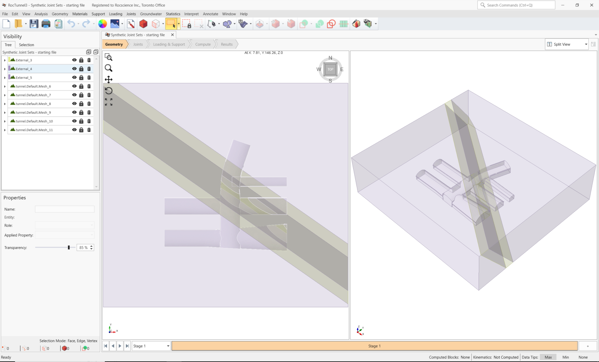
2.3 External Geometry
The External consists of six (6) excavated tunnel pieces assigned with "No Material", two (2) rock mass pieces assigned with Zone 1 material, and one (1) rock mass piece assigned with Zone II material.
2.4 Joint Properties
Review Joint Properties.
- Select Joints > Define Joint Properties or click on the Define Joint Properties
 icon in the toolbar.
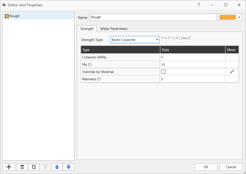
 - The Rough joint property has:
- Under the Strength tab:
- Strength Type = Mohr-Coulomb
- Cohesion = 0 MPa
- Phi = 30 deg
- Override by Material = OFF
- Waviness = 0 deg
- Under the Water Parameters tab:
- Water Pressure Method = Dry
- Click Cancel to exit the dialog.
3.0 Adding Synthetic Joints
In this example, we will be defining synthetic joints sampled using set statistics data from DIPS. For a given Synthetic Joint Property, the following distributions are specified:
- Orientation (i.e., dip and dip direction)
- Spacing (i.e., distance between adjacent joints in a set)
- Radius
With the orientation, spacing, and radius distributions, the user then defines the traversal path as a polyline on which the X, Y, Z center location of each joint is sampled, according the spacing. For each joint, the orientation and radius is sampled according to their respective distributions. Like Measured Joints, Synthetic Joints are also modelled as a planar disk.
3.1 Define Synthetic Joints
While in the Joints workflow tab:
- Select Joints > Define Synthetic Joints

The Define Synthetic Joint Properties dialog contains a list of all defined synthetic joint properties. Each synthetic joint property is defined by distributions of Joint Orientation, and Radius and Spacing. A different Joint Property can be assigned to each joint using the Joint Properties defined in Define Joint Properties dialog. For this demonstration, we will be importing the set statistics data directly from a DIPS file containing 4 joint sets.
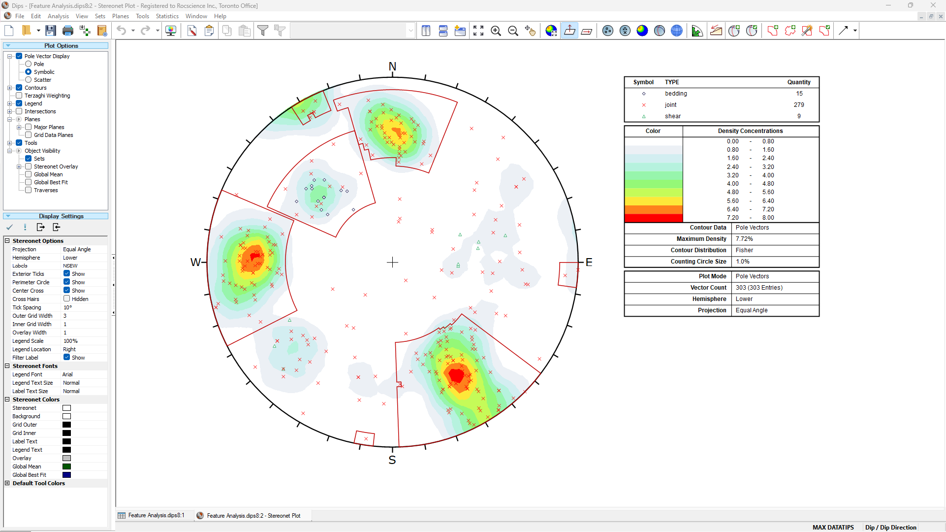
- Click Import From DIPS

- In the Open dialog, select the Feature Analysis.dips8 file from the Tutorials > Synthetic Joint Sets folder and click Open.
- In the Import Synthetic Joints From DIPS dialog:
- Set Terzaghi Weighting = Unweighted. See the Terzaghi Weighting topic from the DIPS User Guide for more information. A listing of Joint Sets from the DIPS file is shown with Name, Set ID, the mean Dip and Dip Direction, and Fisher K.
- Select Overwrite Existing Synthetic Joint Properties. This will overwrite the existing Synthetic Joint Property.
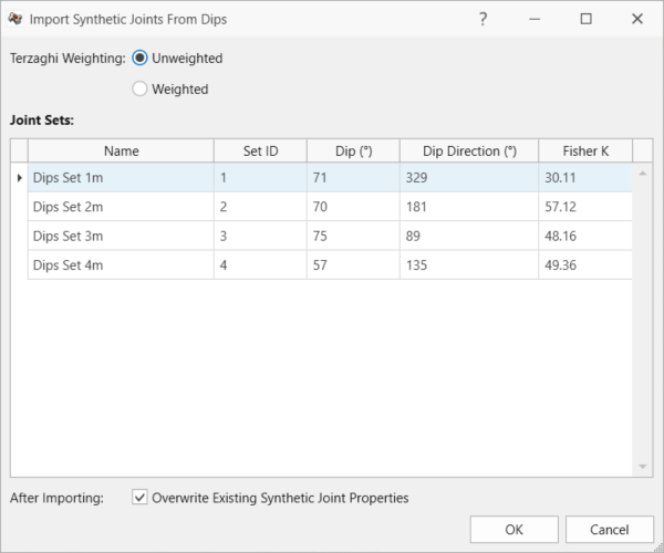
Import Synthetic Joints from DIPS dialog - Click OK to import the four (4) Synthetic Joint Properties from DIPS.
- For each DIPS Set (1m, 2m, 3m. 4m), edit the Radius and Spacing statistics by clicking the Distribution icon to the right of the Mean Radius and Mean Spacing fields. By default, the Distribution will be set to None.
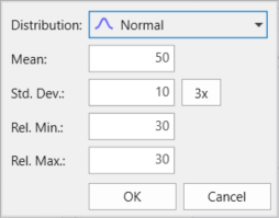
- For DIPS Set 1m:
- Set Mean Radius = 50, Distribution = Normal, Std. Dev. = 10, Rel. Min. = 30. Rel. Max. = 30.
- Set Mean Spacing = 10, Distribution = Normal, Std. Dev. = 2, Rel. Min. = 6, Rel. Max. = 6.
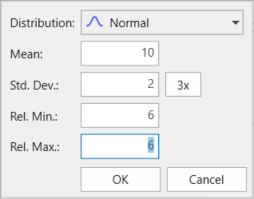
Spacing Statistics Settings - Set Spacing Option = True Spacing. See the Define Synthetic Joints topic for more information on Joint Spacing.
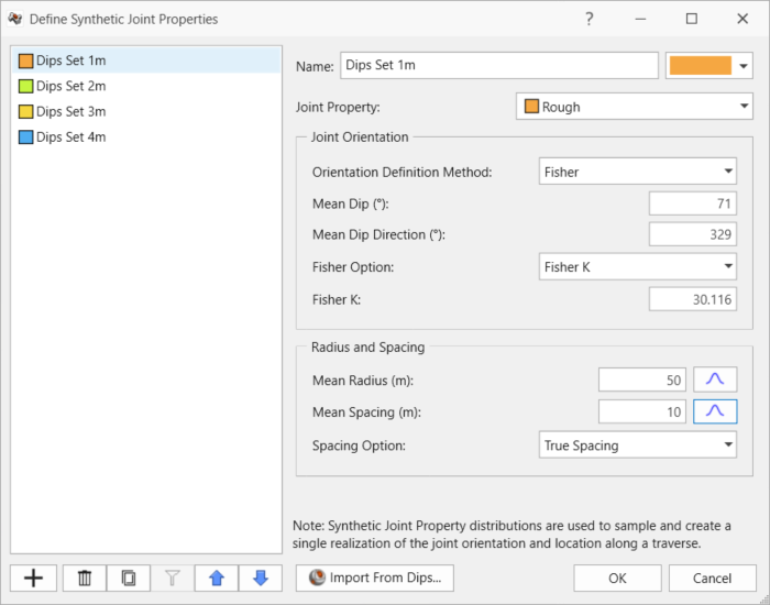
DIPS Set 1m Synthetic Joint Property in Define Synthetic Joints dialog - Repeat Step 6 for DIPS Set 2m, DIPS Set 3m, and DIPS Set 4m.
- Click OK to save the synthetic joint properties and exit the Define Synthetic Joints dialog.
3.2 Add Synthetic Joint Set
Now define the traverse on which the joint locations are sampled based on the spacing of joints (distribution and spacing option).
To add a synthetic joint set:
- Turn off the visibility of External_3, External_4, and External_5 by clicking the visibility icon
 in the Visibility Tree.
 - Select Joints > Add Synthetic Joint Set
- Under the Draw Polyline pane, select Edit Table.
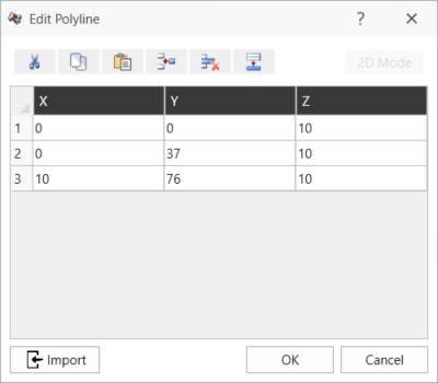
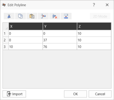
- In the Edit Polyline dialog:
- Specify the X, Y, Z points of the polyline as follows. A quick way to do this is by selecting and copying (CTRL + z) the table of coordinates below with your mouse, and then clicking the Paste
 button in the Edit Polyline dialog:
 - Click OK.
- Click the Done button in the Draw Polyline pane to finalize the polyline.
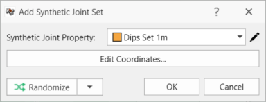
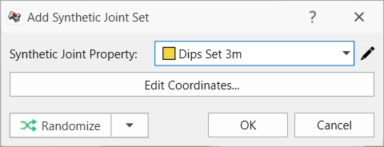
- In the Add Synthetic Joint Set dialog:
- Set Joint Property = DIPS Set 1m.
- Click OK to add the synthetic joint set.
| X | Y | Z |
| 0 | 0 | 10 |
| 0 | 37 | 10 |
| 10 | 76 | 10 |

Select the Synthetic Joint Set entity in the Visibility Tree and the entity will be selected (highlighted red). The following information is shown in the Properties pane:
- Name = Synthetic Joint Set
- Applied Property = DIPS Set 1m
- Transparency = 0%, by default
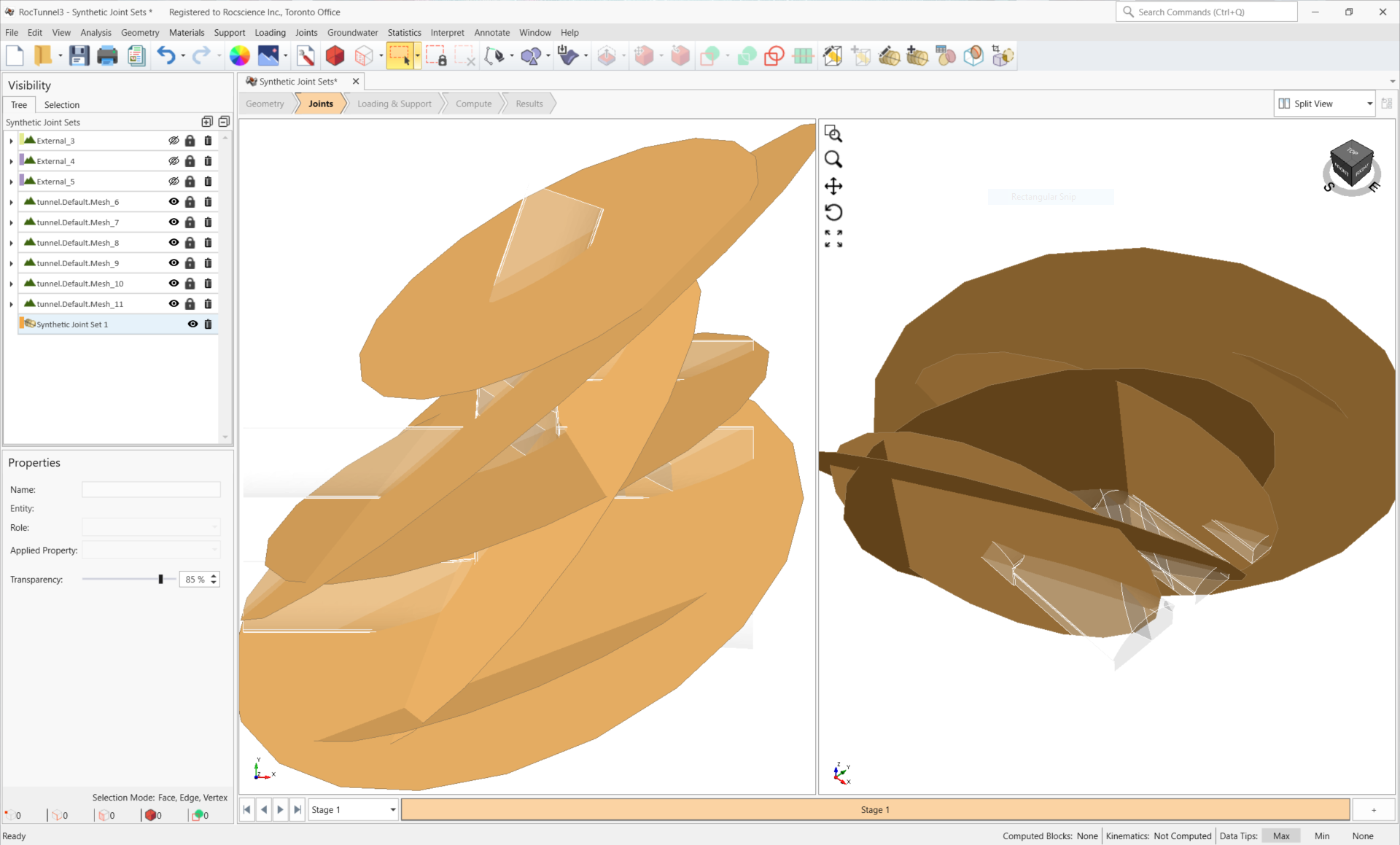
The joints are drawn in the 3D View.
Repeat Steps 1-5 to add the second joint set:
- Select Joints > Add Synthetic Joint Set
- Under the Draw Polyline pane, select Edit Table.
- In the Edit Polyline dialog:
- Specify the X, Y, Z points of the polyline as follows. A quick way to do this is by selecting and copying (CTRL + z) the table of coordinates below with your mouse, and then clicking the Paste button in the Edit Polyline dialog:
- Click OK.
- Click the Done button in the Draw Polyline pane to finalize the polyline.
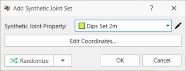
- In the Add Synthetic Joint Set dialog:
- Set Joint Property = DIPS Set 2m.
- Click OK to add the synthetic joint set.
| X | Y | Z |
| 0 | 0 | 10 |
| 0 | 37 | 10 |
| 10 | 76 | 10 |
Repeat Steps 1-5 to add the third joint set:
- Select Joints > Add Synthetic Joint Set
- Under the Draw Polyline pane, select Edit Table.
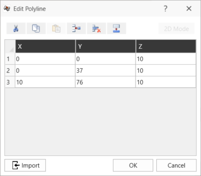
- In the Edit Polyline dialog:
- Specify the X, Y, Z points of the polyline as follows.A quick way to do this is by selecting and copying (CTRL + z) the table of coordinates below with your mouse, and then clicking the Paste button in the Edit Polyline dialog:
- Click OK.
- Click the Done button in the Draw Polyline pane to finalize the polyline.
- In the Add Synthetic Joint Set dialog:
- Set Joint Property = DIPS Set 3m.
- Click OK to add the synthetic joint set.
| X | Y | Z |
| 0 | 0 | 10 |
| 0 | 37 | 10 |
| 10 | 76 | 10 |
Repeat Steps 1-5 to add the fourth joint set:
- Select Joints > Add Synthetic Joint Set
- Under the Draw Polyline pane, select Edit Table.
- In the Edit Polyline dialog:
- Specify the X, Y, Z points of the polyline as follows. A quick way to do this is by selecting and copying (CTRL + z) the table of coordinates below with your mouse, and then clicking the Paste button in the Edit Polyline dialog
- Click OK.
- Click the Done button in the Draw Polyline pane to finalize the polyline.
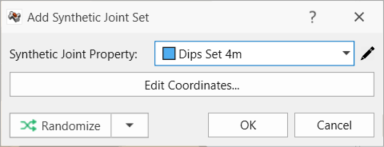
- In the Add Synthetic Joint Set dialog:
- Set Joint Property = DIPS Set 4m.
- Click OK to add the synthetic joint set.
| X | Y | Z |
| 0 | 0 | 10 |
| 0 | 37 | 10 |
| 10 | 76 | 10 |
The joints are drawn in the 3D View.
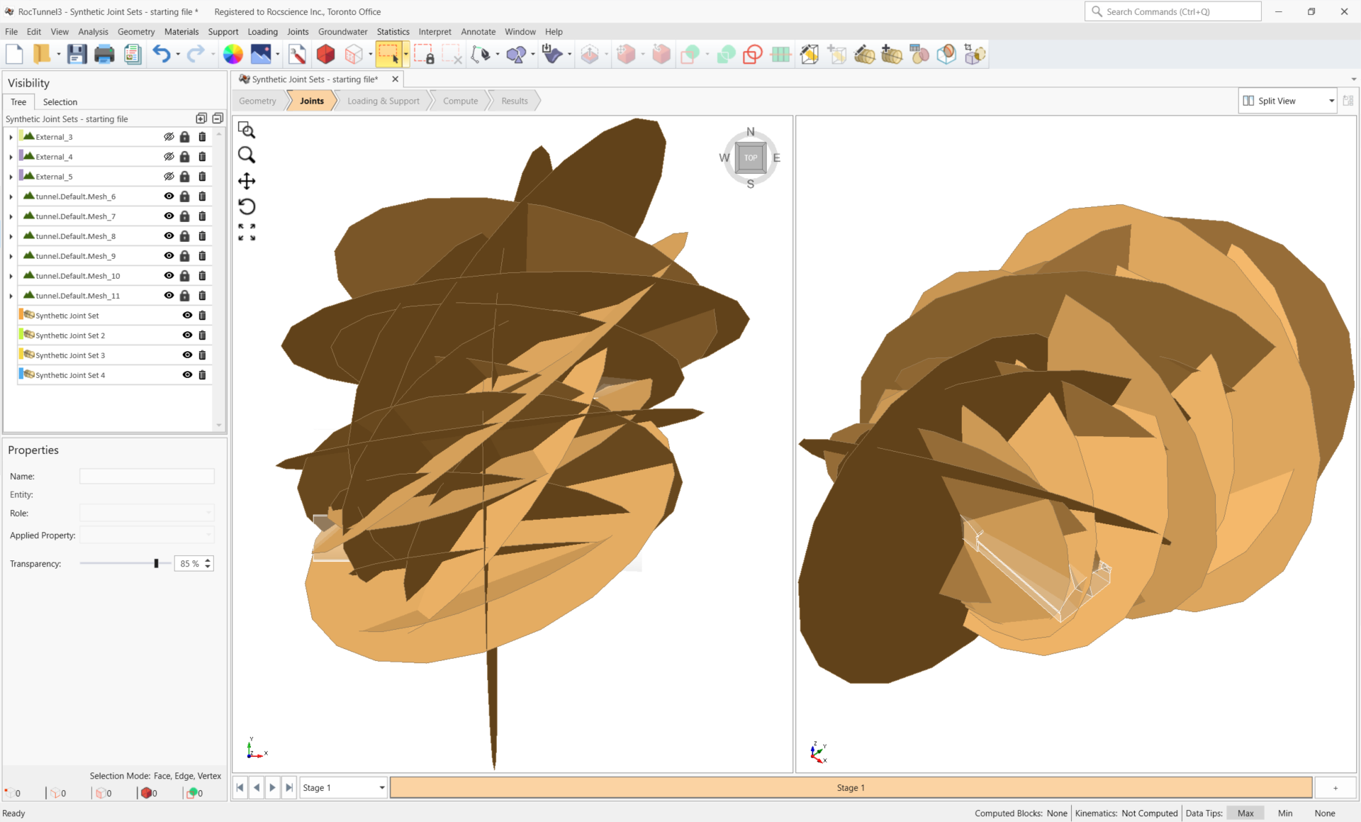
3.3 Joint Colours
By default, all joints are coloured according to the assigned Joint Property colour. In this model all three Synthetic Joint Sets are assigned the same Joint Property (i.e., Rough) and are therefore it is hard to distinguish between the sets.
To colour joints by the Synthetic Joint Property:
- Select View > Display Options

- In the Display Options dialog, navigate to the Joints tab.
- Select Use Synthetic Joint Property Color.
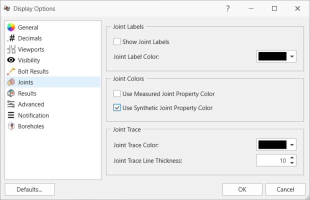
Joints tab in Display Options dialog - Click OK to close the dialog.
The joints are now coloured according to Synthetic Joint Property colours.
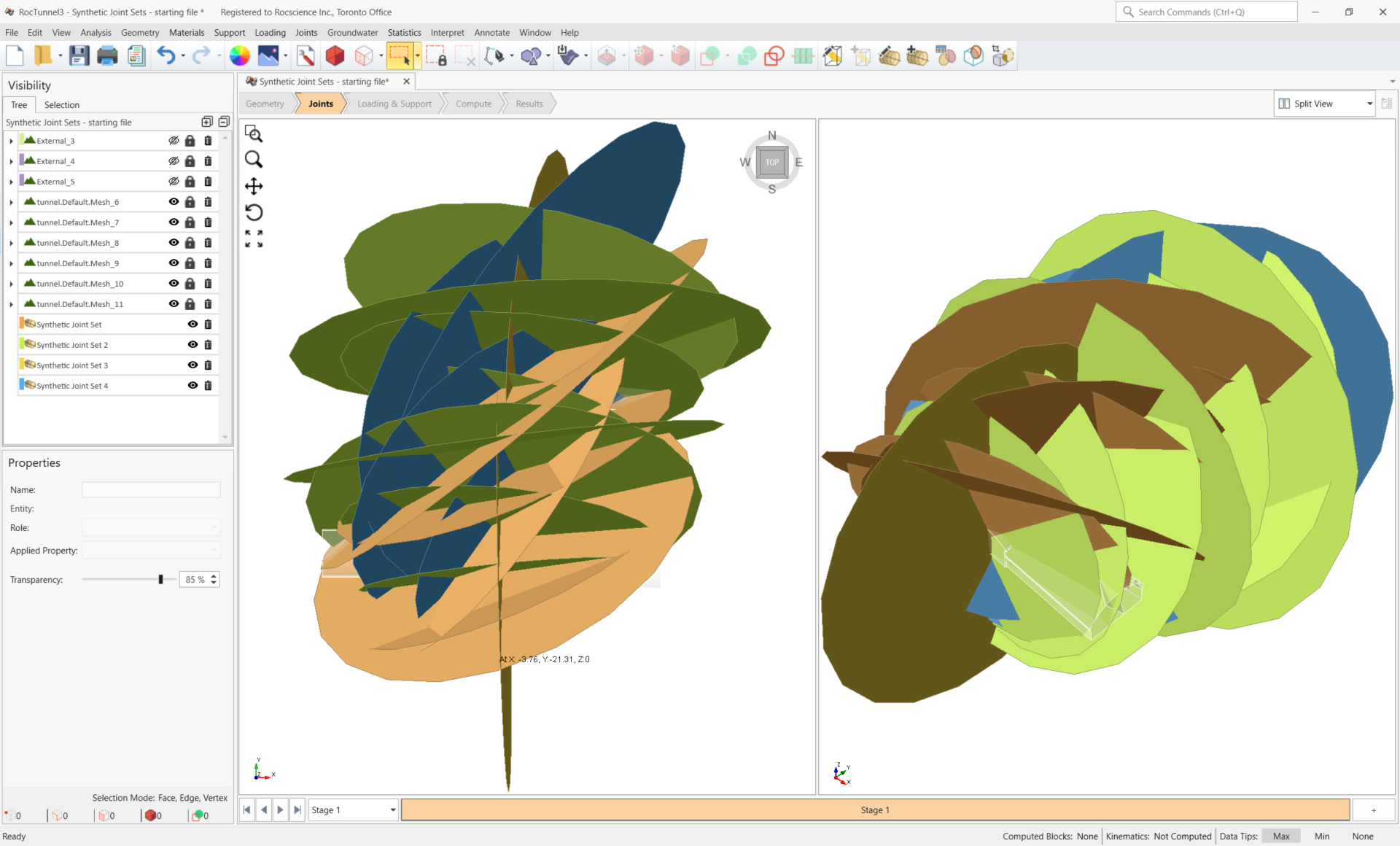
3.4 Synthetic Joint Information
To view a listing of all joints belonging to a Synthetic Joint Set:
- Select any of the Synthetic Joint Set nodes from the Visibility Tree.
- Select Synthetic Joint Information button from the Properties pane or select Joints > View Synthetic Joint Information in the menu.
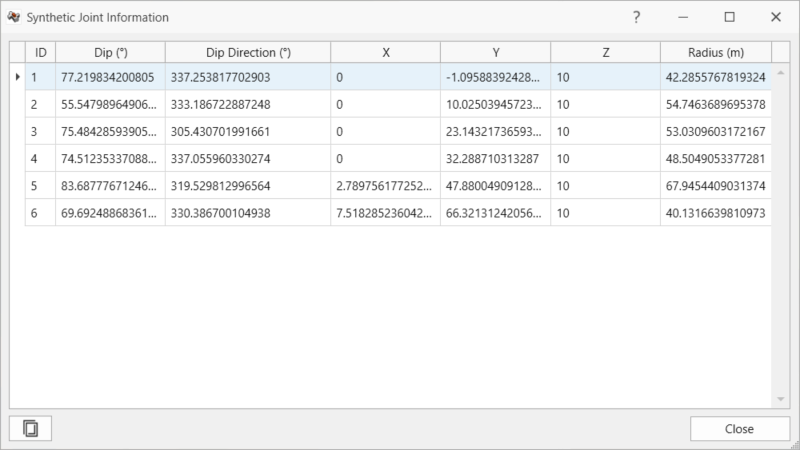
- The Synthetic Joint Information dialog shows a listing of joints in the set with Dip, Dip Direction, X, Y, Z, and Radius columns. The information can be copied by clicking the Copy button at the bottom-left of the dialog.
- Click Close to exit the dialog.
3.5 Randomize Synthetic Joint Sets
Synthetic Joint sampling is NOT a probabilistic analysis using joint orientation, radius, and spacing as random variables. We are only sampling the joints in a joint set once to get variations in joint orientation, radius and spacing across the traverse. In other words, the sampling only represents one realization of the joint set. The joint set sampling is determined according to the statistics defined in the applied Synthetic Joint Property (i.e., Orientation, Radius, Spacing), the Traverse polyline, and the Pseudo-random Seed value (default seed = 10116).
The ability to form of blocks, the removability of blocks, and the kinematics of blocks are extremely dependent on the joint's orientation, persistence, and spatial location. In some cases, a user may want to see different realizations of the Synthetic Joint Sets so that a different statistical sampling of the synthetic joints are generated and potentially a different collection of blocks.
To regenerate the sampling for a Synthetic Joint Set:
- Select any of the Synthetic Joint Set nodes from the Visibility Tree.
- Under the Properties pane, select Edit to edit the geometry.
- In the Edit Synthetic Joint Set dialog:
- Click the Randomize button to randomly pick a new Pseudo-random Seed value. Note that the joints in Synthetic Joint Set 1 have been sampled again using the same distributions but different randomization.
- Repeatedly click the Randomize button a few times to get different realizations.
- Select the dropdown from the Randomize button and select Edit Random Seed. The Random Seed dialog shows the current
Pseudo-random Seed value.
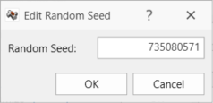
Edit Random Seed dialog - Select OK to close the Edit Random Seed dialog.
- Select the dropdown from the Randomize button and select Reset Random Seed. The Pseudo-random Seed value is reset back to the default seed value of 10116. Joint Set 1 will be sampled identically to the initial realization of the joints.
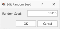
Edit Random Seed Dialog showing default seed value - Click OK to close the Edit Synthetic Joint Set dialog.
4.0 Compute
RocTunnel3 has a two-part compute process.
4.1 Compute Blocks
The first step is to compute the blocks which may potentially be formed by the intersection of joints with other joints and the intersection of joints with the free surface.
To compute the blocks:
- Navigate to the Compute workflow tab

- Select Analysis > Compute Blocks or click the Compute Blocks
 icon in the toolbar.
As the compute is run, the progress bar reports the compute status. Once the compute is finished, the Results node is added to the Visibility Tree and All Valid Blocks are shown in the 3D View. The Results node consists of the collection of valid blocks and the socketed slope and socketed excavation (by default, Show Socketed Slope is OFF). The original External and Synthetic Joint Sets visibility is turned off.
The blocks are coloured according to the Block Colors option. The Block Colors settings can be edited in the Results node's Property pane or in the Display Options dialog. By default, Block Colors is set to Random Colors, which colours each adjacent block a different colour to be able to easily distinguish between different blocks. The program's default Block Colors can be changed in the Display Options dialog.
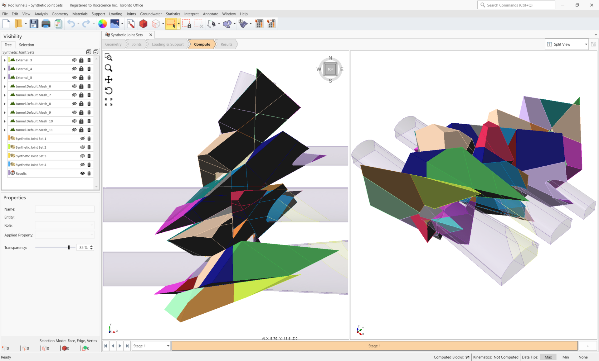
For this tutorial, 53 blocks have been computed (some may be invalid). This is indicated by the "Computed Blocks: 53" on the status bar at the bottom-right of the application window.
Compute Blocks only determines the geometry of the blocks. In order to obtain other information such as the factor of safety, Compute Kinematics needs to be run.
4.2 Compute Kinematics
The second and final compute step is to compute the kinematics for each of the valid blocks, including the removability, forces, and factor of safety.
To compute the block kinematics:
- Ensure that the Compute workflow tab is selected.
- Select Analysis > Compute Kinematics or click on the Compute Kinematics
 icon option in the toolbar.
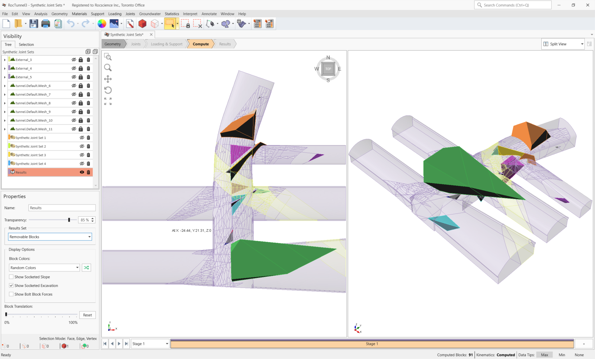
As compute is run, the progress bar reports the compute status. By default, after Compute Kinematics is run, only Removable Blocks are shown.
5.0 Interpreting Results
Once both blocks and kinematics are computed, all block results can be viewed in a table format.
5.1 Block Information
To view all block results:
- Navigate to the Results workflow tab

- Select Interpret > Block Information or click on the Block Information
 icon option in the toolbar.
Visualizing blocks can be difficult when the excavation extents are large compared to the block extents.
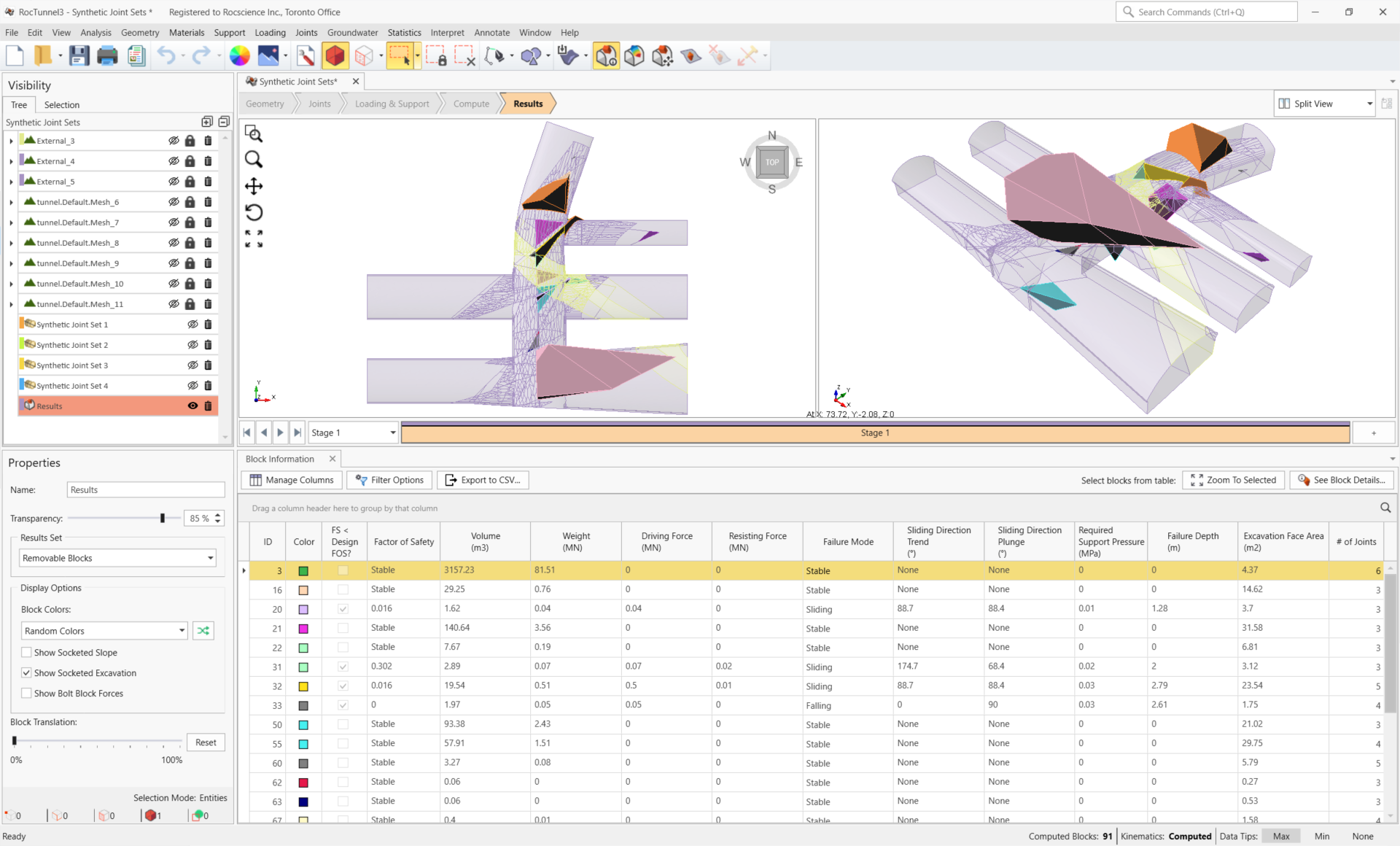
The Block Information pane shows the collection of blocks according to the Results Set settings. The Results Set shown can be selected in the Results tab of the Display Options, or the Properties pane for the Results node. Currently, Removable Blocks are listed.
By default, the first row is selected. The corresponding selected block is highlighted in PINK in the 3D CAD View.
To unhighlight the block:
- Left-click anywhere in the 3D CAD View where there are no blocks.
Visualizing blocks can be difficult when the excavation extents are large compared to the block extents.
To zoom to a selected block in Block Information pane:
- Select a row in the Block Information pane.
- Click Zoom to Selected
 (located in the top right of the Block Information pane).
TIP: Alternatively, double left-click on a row in Block Information to zoom to the block in 3D CAD View. When selecting a block from the 3D CAD View, the corresponding row is automatically selected in the Block Information pane.
6.2 Contour Blocks
Not only are the magnitudes of critical values (such as the block's factor of safety or weight) important to be aware of, the location also matters. The Contour Blocks option allows the user to plot a safety map of various block metrics so that the range of values can be visualized over the excavation.
To show block contours:
- Select Interpret > Contour Blocks or click on the Contour Blocks
 option in the toolbar.
 - From the Legend pane on the right, select Factor of Safety from the drop down.
- All the blocks are coloured according to the Factor of Safety contour legend. The minimum Factor of Safety blocks are contoured RED while the blocks with Factor of Safety > 5 are contoured BLUE. The Contour Options can be customized. See the Contour Options topic for more information.
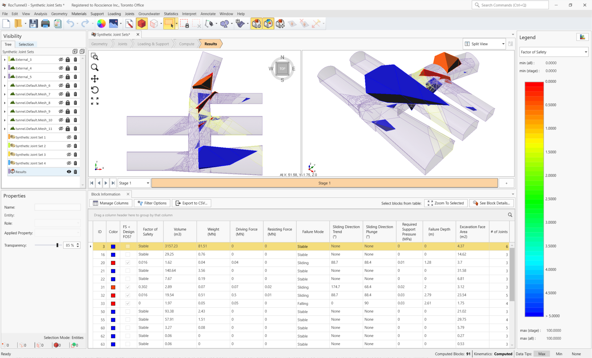
From this heat map of Factor of Safety, locations with the lowest factors of safety and highest failure risk can be identified. The lowest Factor of Safety Blocks are colored in RED and ORANGE. These blocks occur on the roof of the tunnel spanning North-to-South. Typically, Removable blocks on the roof of an excavation will have little to no Resisting Force if unsupported.
Let's view some Failed Blocks in detail:
- Double click Block 83 from the Block Information pane. Note that Sliding Direction Plunge is 90 degrees (in the direction of gravity) and the Failure Mode is Falling which means that the block has lost contact with all joint faces, and therefore zero Resisting Force is provided by shear.
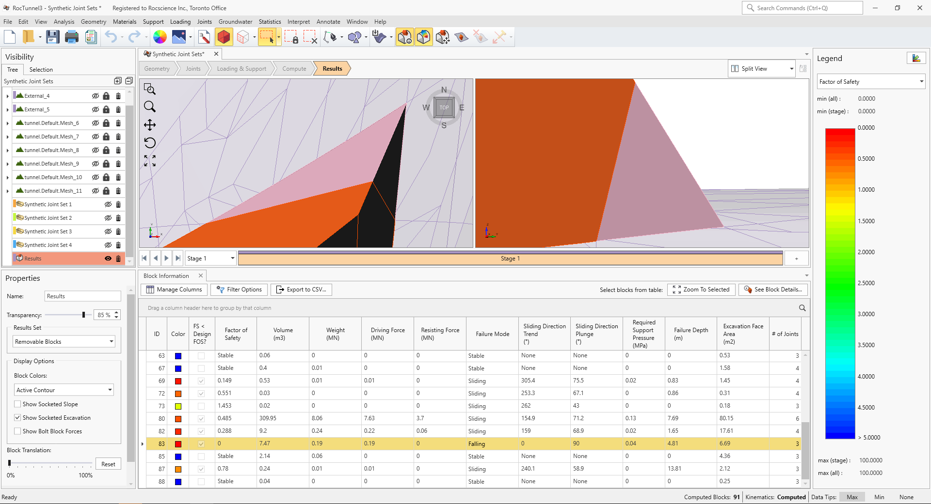
Block 83 in Block Information - Double click Block 80 from the Block Information pane. Note that the Failure Mode is Sliding but insufficient shear resistance along the sliding joint is provided.
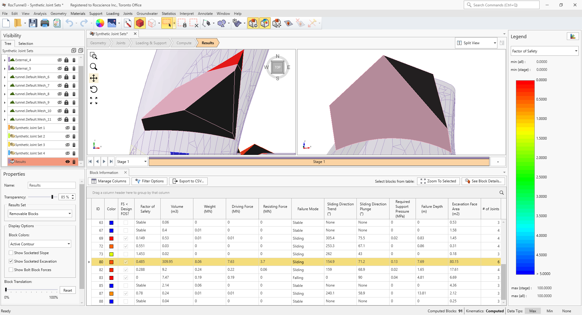
Block 80 in Block Information - Click See Block Details
 (for Block 80).
In the Detailed Block Information dialog, note that the Sliding Joints are on joints 3 and 4 which have non-zero Normal Forces and non-zero Shear Strength. The block loses contact with all other joints when sliding occurs (i.e., zero Normal Force and zero Shear Strength). The Sliding Direction Trend and Plunge is along the line of intersection of the joints 3 and 4.
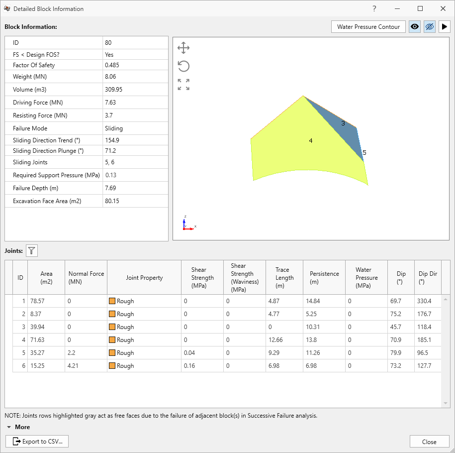
Block 80 in Detailed Block Information dialog - Click Close to exit the Detailed Block Information dialog.
Stable blocks or blocks with large Factors of Safety are colored BLUE. Block 3 is flagged as Removable (since it daylights on the ground surface) but is Stable since it cannot fall inside the excavation in the direction of the Driving Force (i.e., downward in the direction of gravity). Likewise, the blocks on the floor of the tunnels are also Removable but Stable.
This concludes Tutorial 2.