RS2 Compute UI

The RS2 Compute UI allows users to select files to run and displays the key data for the current simulation. It appears when Compute or Compute (groundwater only) is launched, which whether is from the Analysis menu in RS2 modeler, or as a standalone program (feawin.exe) from the installation folder.

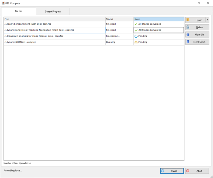
There are two tabs in RS2 Compute UI. The File List tab allows users to open and organize RS2 files, and the Current Progress tab presents general information and graphs for selected key data for users to monitor the data change over the simulation.

File List

Open Files to Compute

If users want to select RS2 files to compute from the RS2 Compute UI:

1. Select the File List tab.
2. Select Open to open one or more files. A Windows Open file dialog will display. RS2 files have a *.fez filename extension. Select the .fez file(s) you want to compute, click Open.

   
   Note: Users can click on the expandable button beside “Open” to choose files from Examples folder, Tutorials folder, and previous files. Users can also drag and drop files to the File List section.

3. The selected files will be added to the file list with:
   1. Filename - when the mouse is hovered over the filename, the full path of will appear.
   2. Status – processing, queueing, did not converge, or finished.
   3. Note – detail description for the status

      
      Note: The number of files on the list will show in a sentence below the file list.

4. Select the Compute button to perform the finite element analysis for the listed files following the listed order.
5. Users can pause the simulation with the Pause button , and Resume .
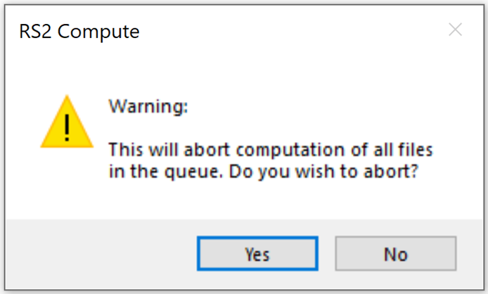
6. Users can abort the simulation with the Abort button . A warning dialog will pop up.



7. Click Yes to confirm abort. Then users can select other file(s) to compute, or exit the UI with the Exit button .

Delete Files

Select the files on the file list to highlight, and then select the delete button to remove them from the file list.

Edit Files

Use the Move Up and Move Down buttons to rearrange the file sequence on the list.

Current Progress

The Current Progress tab allows users to monitor the progress of the simulation and overview the development of selected key data. All data displayed can be found in RS2 modeler or RS2 Interpret after the computation. The Current Progress tab contains six sections: Current Progress, General Information, Stage Information, System Information, Convergence Graphs, and History Graphs . The General Information, Stage Information, and System Information can be expanded/minimized by clicking on the expandable button on top of the section.

Current Progress

This section provides progress status information, including:

• Input File name.
• Elapsed time - since the simulation started.
• Elements - total mesh element number of the model.
• DOF – degree of freedom, which will change by stage.
• A progress bar in terms of Stage.
  If a Shear Strength Reduction (SSR) analysis is carried out, the current SRF value that is used to alternate the material properties of the model will display on top of the Stage progress bar.
• A progress bar in terms of Load Step.
• A progress bar in terms of Time Step.

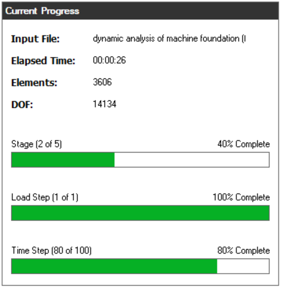(Multi-stage model without SSR analysis)

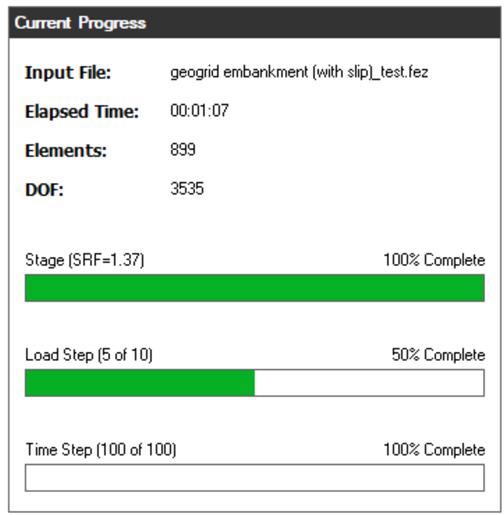(Multi-stage model with SSR analysis)

General Information

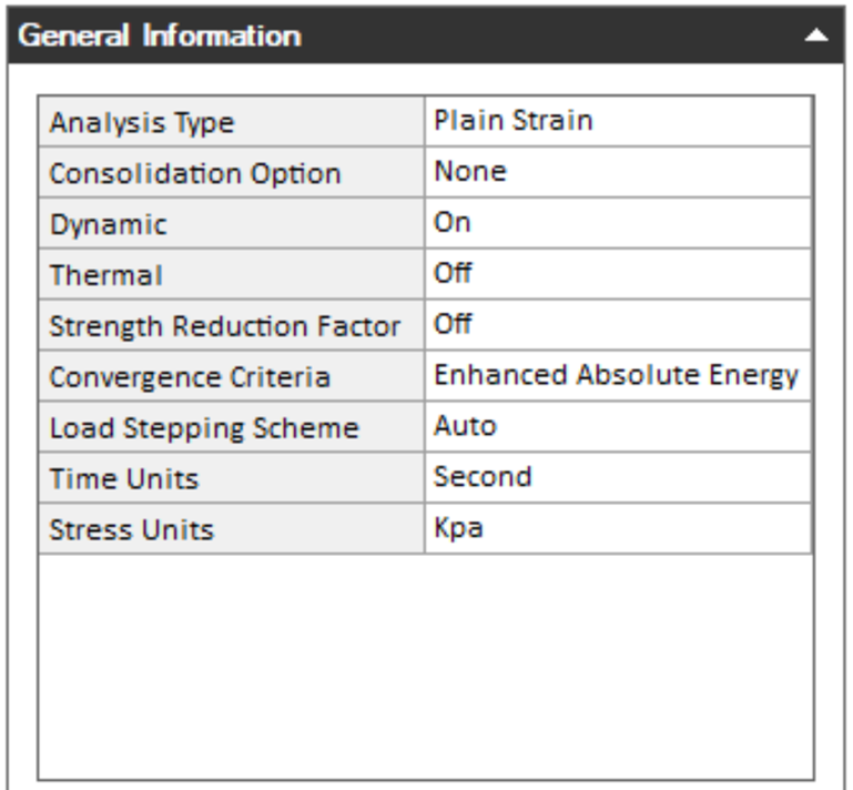
This section provides general information of the model, including the Analysis Type, Consolidation Option, Dynamic, Thermal (coming soon), Strength Reduction Factor, Convergence Criteria, Load Stepping Scheme, Time Units Stress Units. The information can be found in Project Setting.

Stage Information

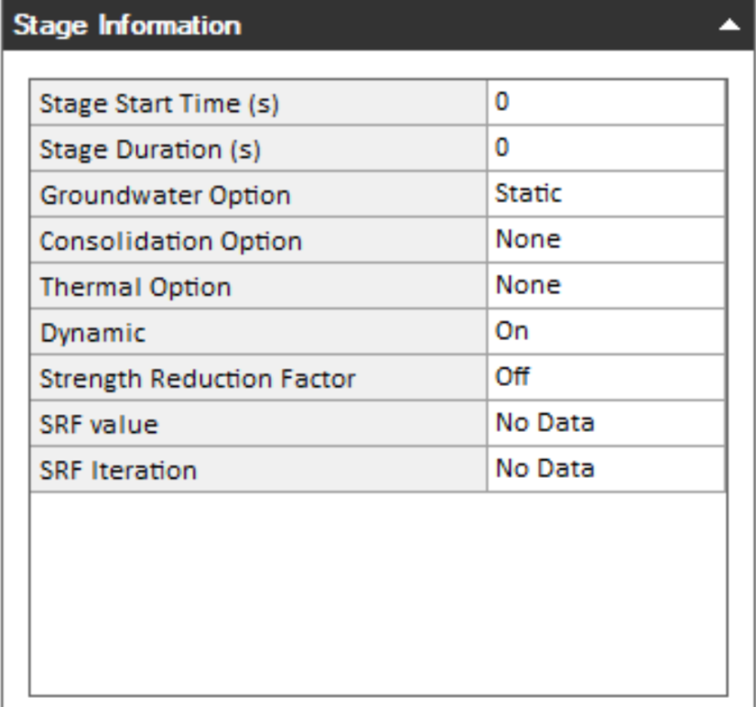
This section provides information for the current running stage, including the Stage Start Time (s), Stage Duration (s), Groundwater Option, Consolidation Option, Thermal Option (coming soon), Dynamic, Strength Reduction Factor, SRF value, and SRF Iteration.

System Information

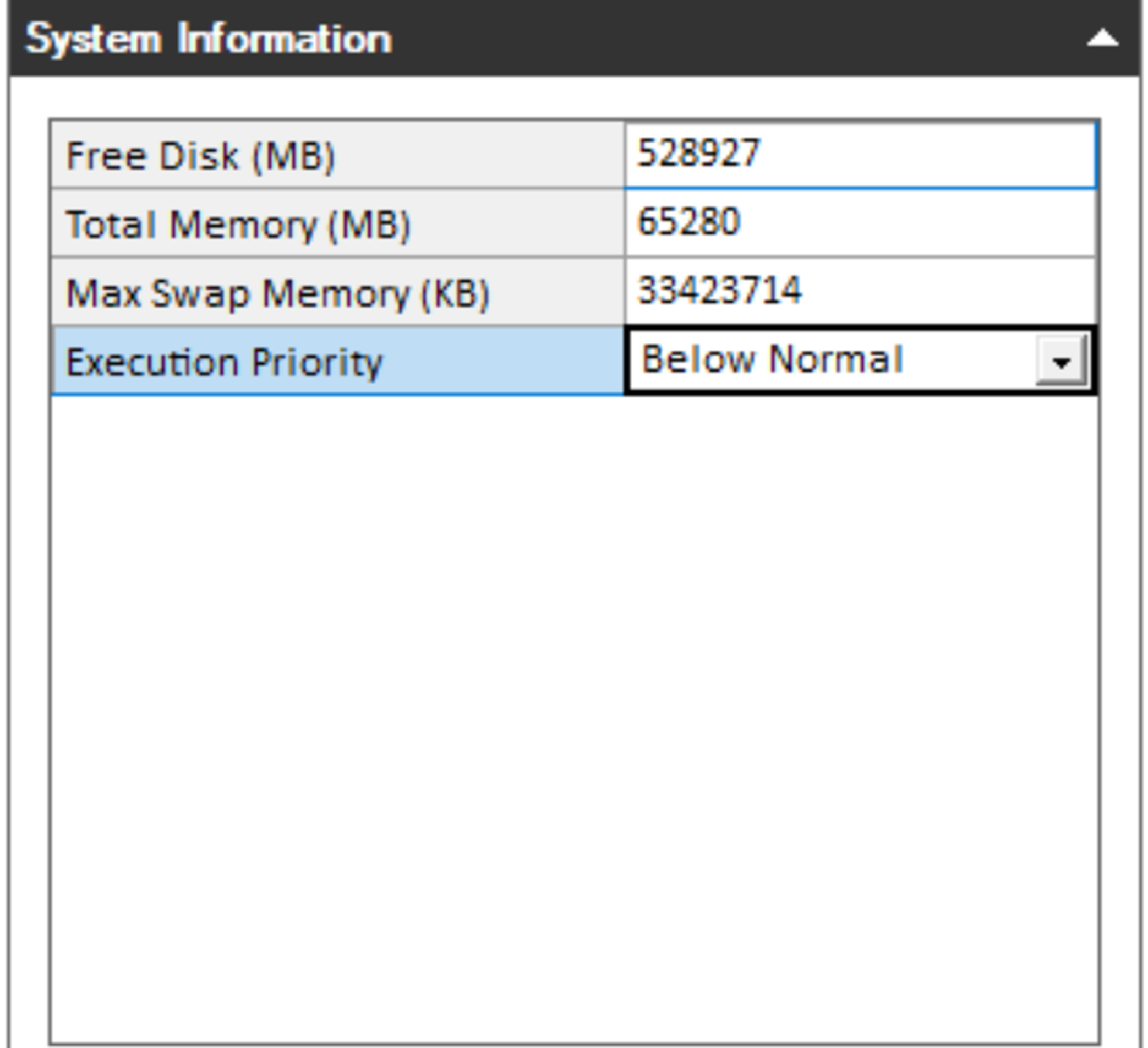
This section provides system information for the file, including Free Disk (MB), Total Memory (MB), Max Swap Memory (KB), and Execution Priority. The Execution Priority indicates the priority level of RS2 program compared to other programs. Users can adjust the execution priority using the dropdown bar.

Convergence Graphs

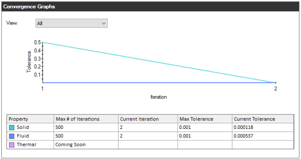
The convergence information for the finite element stress analysis will be presented graphically. The Tolerance versus the Iteration for the current load step will be plotted. The graph shows the development over one load step of the calculation. Each data point represents the calculated tolerance for the current iteration. The tolerance is calculated based on the selected convergence criteria that shown in the General Information. The Y axis is dynamic, that the flexible range helps to better visualize the data variation.

For one iteration, if the current tolerance is less than the maximum tolerance value, then the solution is considered to have converged. A maximum number of iterations can be performed at each load step for the stage.

Users can plot the graph for one or all material properties (solid, fluid, and thermal). The relevant convergence parameters for each material property are summarized in a table:

• Max # of Iterations: the defined maximum number of iterations for each load step.
• Current Iteration: the current iteration number out of the maximum number of iterations.
• Max Tolerance: the defined maximum tolerance value for a load step.
• Current Tolerance: the calculated tolerance value for the current iteration.

History Graphs

The section displays the development of displacement, pore pressure, and temperature graphically. Two types of data can be plotted:

1. Maximum Values

Select Plot = Max from the dropdown bar. Select the time reference as the Y-axis from one of the three options: Load Percentage Stage, Stage Number, and SRF. The history graphs for the Maximum Displacement, Delta Pore Pressure, and Delta Temperature will be computed respectively.

2. History Query

History Graphs for History Query allow users to observe the data development at a specific location over the simulation. To enable History Graphs for History Query, one or more History Query points must be defined prior in the modeler with the Add History Query option.

Select one History Query point (the default name will be HQ#) from the dropdown bar beside Plot. Select the time reference as the Y-axis from one of the three options: Load Percentage Stage, Stage Number, and SRF. The history graphs for the Displacement, Pore Pressure, and Temperature of the History Query location will be computed respectively.

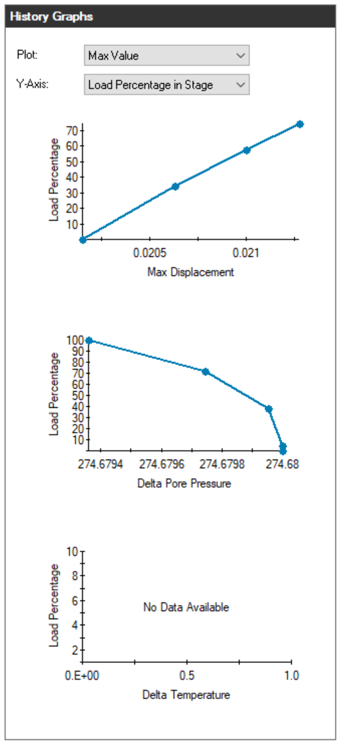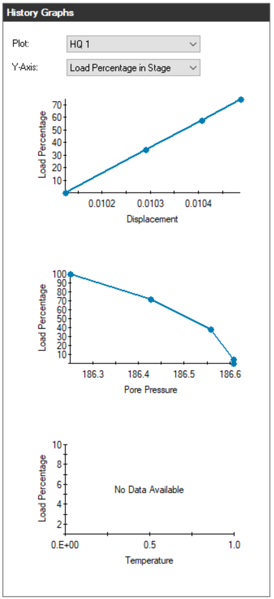History Graphs - Max Values	History Graphs - History Query