Block Model

1.0 Introduction

The block model feature allows you to import a block model database to RS3 project, with each block containing its associated material properties. This tutorial provides an example case of integrating this feature for geomechanical modeling exercise. It incorporates a guidance to import the block model, use material properties stored in the database, and a numerical analysis with an open pit model. Furthermore, an advanced section is included, which introduces importing the Slide3 project that has a block model, and the comparison between results computed from Slide3 and RS3.

The block model database used for this tutorial consists of data with Mohr Coulomb and Generalized Hoek-Brown strength properties of different rock mass units covering the area under investigation. Based on the projected region of disturbance due to the open pit excavation, reduced strength properties are recorded in the database, within some depth from the slope.

All tutorial files installed with RS3 can be accessed by selecting File > Recent > Tutorials folder from the RS3 main menu. The initial file of the tutorial can be found in Block Model - starting file.rs3v3 file and the finished tutorial can be found in the Block Model - final.rs3v3 file.

2.0 Starting the Model

1. Select File > Recent > Tutorials.
2. Open the starting file Block Model - starting file.rs3v3.

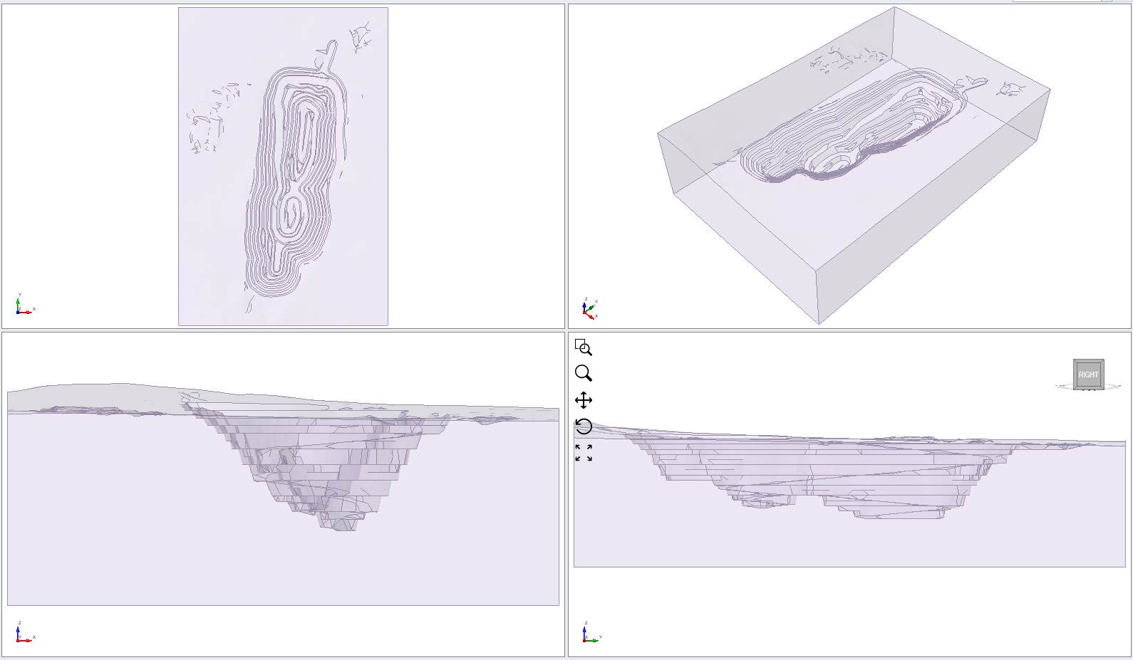
The project file should already contain the external geometry of an open pit mine that has “Master Material” property assigned. The model is meshed and have boundary condition applied to conduct the slope stability analysis. Toggle the Eye icon to hide/unhide under Visibility Tree to check out the mesh distribution and boundary condition setting. The project should have the units set up as Metric, stress as MPa from Project Settings and open pit geometry ready to be used for the analysis.

3.0 Import Block Model

This section provides a procedure to import the block model into the RS3 project. RS3 can consume the block model file in .txt or .csv format. For more information on the block model database format, please visit the documentation page here.

1. To start the importing process, select Materials > Import Block Model.
2. Select the Master Material from the material property list to assign for the master material and click OK.
   
   
3. Enter C:\Users\Public\Documents\Rocscience\RS3 Examples\Tutorials\Block Model - starting file > select Block Model Database.csv (default directory where Tutorials are saved) > Click Open to import.
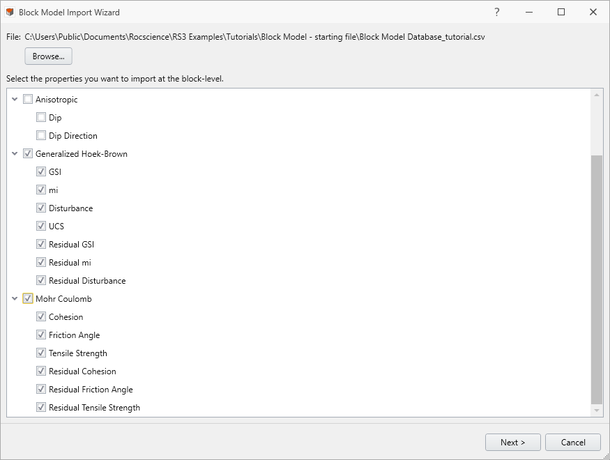
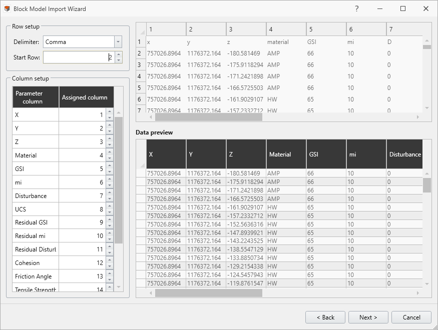
4. The Block Model Import Wizard will be prompted. Select all Generalized Hoek-Brown and Mohr-Coulomb parameters, then select Next.
   
5. Under Row Setup, assign the Start Row (the row of which the RS3 start reading from the database) as 2. The csv file already has the location (x, y, and z), material ID (Material), and strength parameter data (selected Mohr-Coulomb parameters) sorted in the order as required by the import wizard.
   
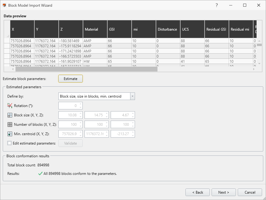
6. Select Next to prompt the block model estimation/rendering part. Select Estimate, the importer computes the block configuration and shows the total number of blocks generated from the database and the conformity test results.
   
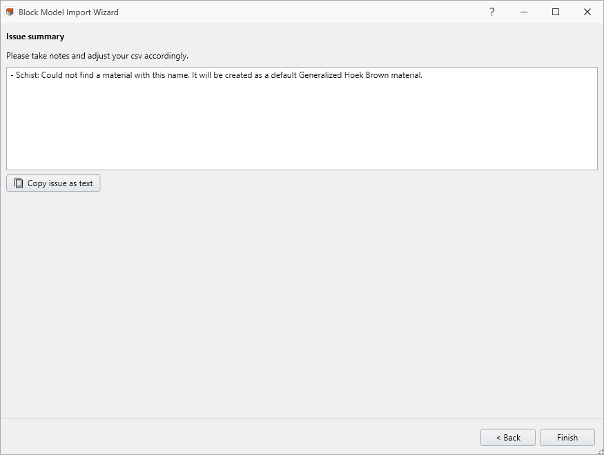
7. Select Next to go to the Issue Summary. In this case, the material “Schist” is noted here, since no material with a matching name exists in the project.
   
8. Select Finish to complete the import process.
9. The visualization of the block model is rendered with the formation of entity Block Model, which shows the regional coverage of blocks, color coded with different material ID.
   
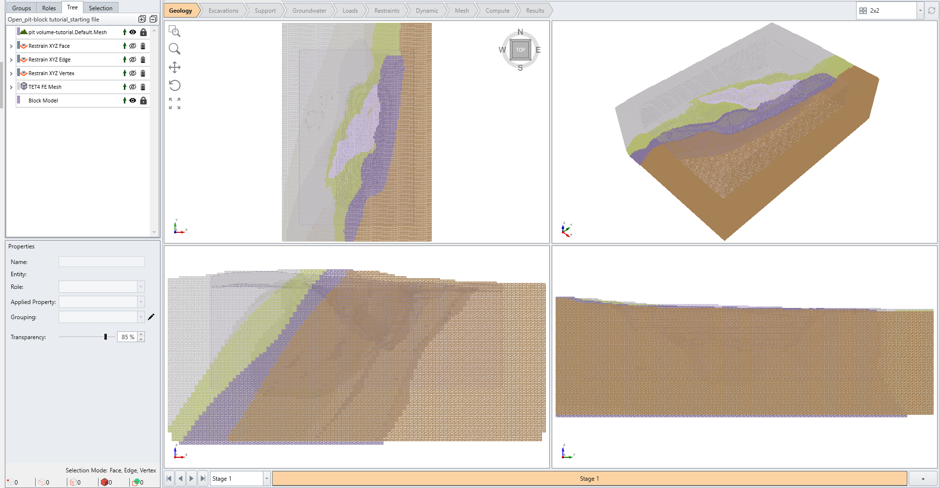
10. Hide the Block Model entity by selecting the eye icon under the Visibility tree and select pit volume-tutorial.Default.Mesh external volume entity.
11. Under Properties pane, select Block Visibility View option and reduce the transparency to 0. This will show the material property that would be applied based on the external volume triangulation. However, note that the geometry triangulation is typically much coarser than the mesh distribution and hence the coloration is not an accurate representation of material assignment for consistent elements.

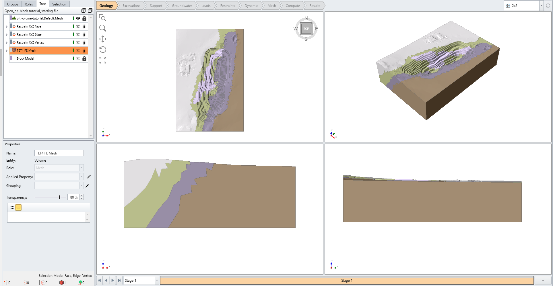
The projection of block model property on the external volume is only done for the those that have Master material applied. Surface selection cannot be done

4.0 Material Properties

1. Select Materials > Define Materials
2. Select Master Material from the list of materials, which is assigned as the host of imported block model data.

A master material has a unique set of properties tab. The Block Database tab shows a summary of the information on imported block model, including block information, list of child materials, and statistics summary of all imported material parameters. For more information, please visit the documentation page here.

1. Select the AMP material property from the left pane. Select the Strength tab and select the Block Data check boxes for all of the options listed:
   
2. Repeat the Block Data selection for Mohr-Coulomb strength parameters for both the HW and FW material properties.
3. Select the ORE material property form the left pane. Set the Failure Criterion as Generalized Hoek-Brown, and the Material Type as Plastic. Select the Block Data check boxes for all parameters:
   
4. Select Schist, the newly created child material. Its default Failure Criterion is Generalized Hoek-Brown.
5. Apply the following properties to the Schist property:

Properties Tab	Material Parameters	Value
Initial Conditions	Unit Weight (MN/m3)	0.024
Stiffness	Poisson’s Ratio	0.3
	Young’s Modulus (MPa)	6143.72

6. Under the Strength tab, set the Material Type to Plastic and select the Block Data check box for all parameters (same settings applied to ORE).
7. Select OK to confirm all changes made to material properties and close the Material Properties dialog.

5.0 Computing Results

Next, select the Compute workflow tab

From this tab, we can compute the results of our model. Before commencing the stress analysis computation, it is recommended to save the final model as a separate file so that you can access the original file anytime.

To save the file before computing:

1. Select File > Save As
2. Then, select Compute > Compute

6.0 Result Interpretation

Select the Results workflow tab to see the modeling results

6.1 Failure Distribution

1. Select Interpret > Yielded Elements > Pick Yielded Elements
2. Select Shear and Tension under Solid Elements.
   
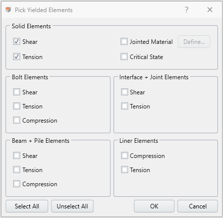
3. Click OK. The location of yielded elements and their failure are revealed on the viewport.
   

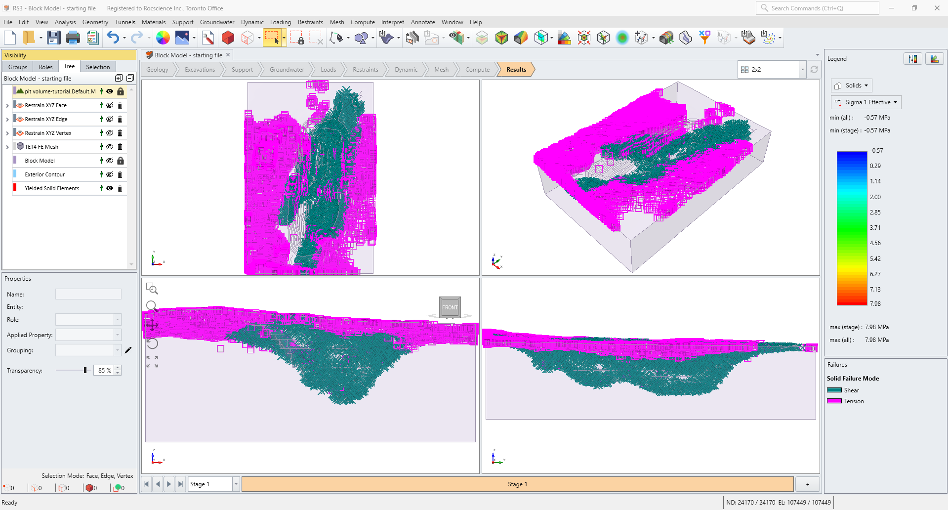
6.2 Stress/Deformation Contour

1. Hide Yielded Solid Elements under the Visibility Tree.
2. Hide external pit volume-tutorial.
3. Select Interpret > Show Exterior Contour.
4. By default, Major Principal Stress is displayed.
   
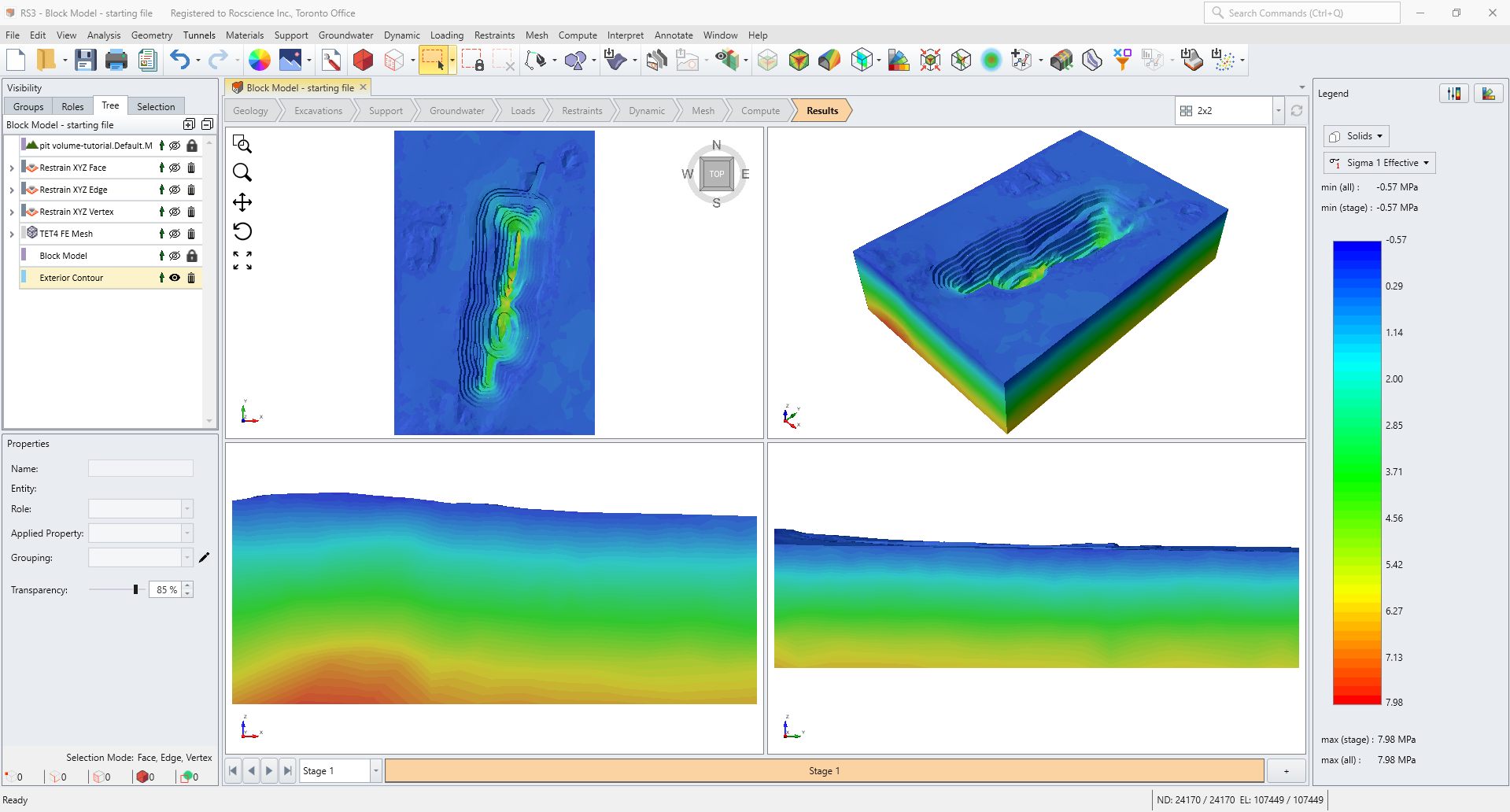
5. Select Result Data Type > Solid Displacement > Total Displacement to see overall deformation distribution on the slope surface
   

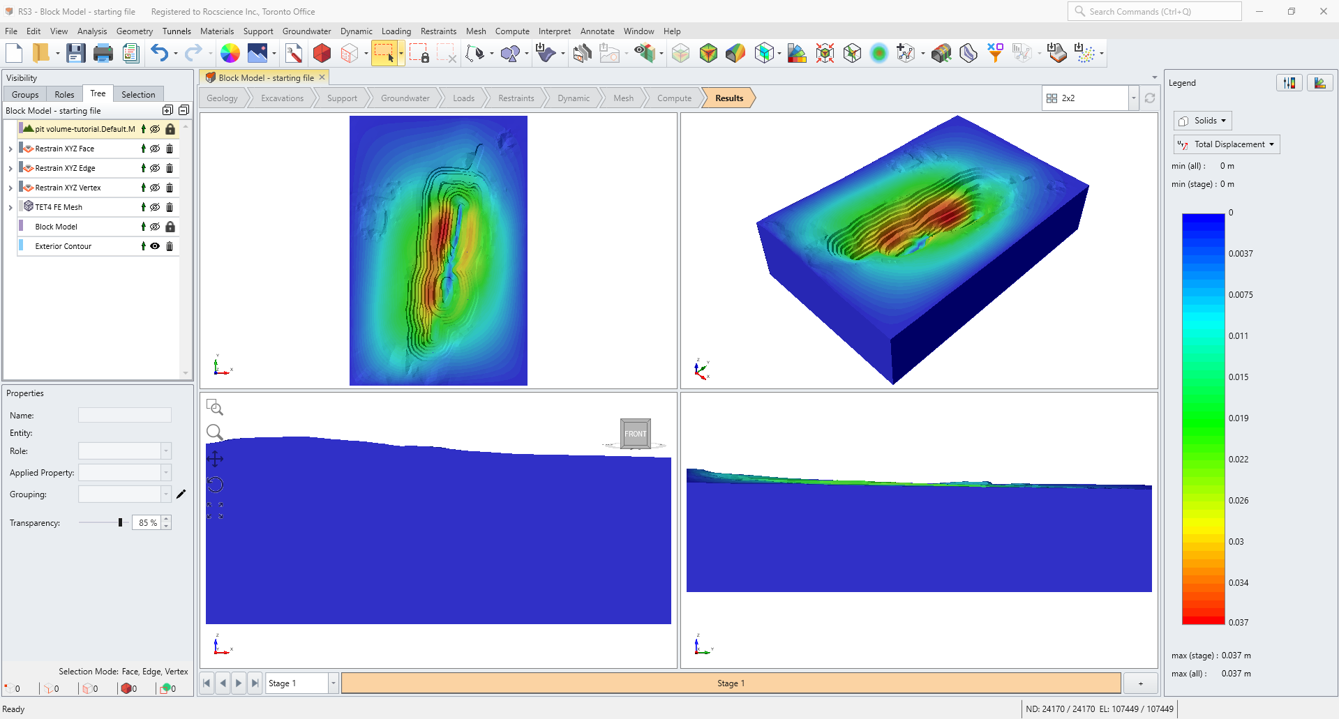
This concludes the main part of the tutorial.

7.0 Additional Exercise

In this section demonstrates importing to RS3 the Slide3 project that has the block model. The Slide3 model was applied with similar setup as the RS3 model used for the main part of this tutorial, including the block model, slope geometry, and material properties. However, this model has a search limit defined to limit the slope surface generation within the region enclosed by the search limit.

The prepared Slide3 project (Block Model-RS3 tutorial.slide3m2) can be found in Block Model – final folder in RS3 Tutorial folder (File > Recent > Tutorials).

7.1 Import Slide3 with block model to RS3

1. Select File > Import > Import Slide3 Project and open Block Model-RS3 tutorial.slide3m2 project. This process sets the RS3 project file to conduct SSR analysis in default with all imported materials set to be plastic.
2. When the import wizard is prompted, deselect Generate Mesh and set Auto Restraints: None.
   
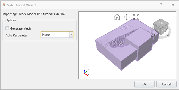
3. Upon the completion of import, a new RS3 project file is created with block model and pit volume as in Slide3 project file.
   [Please ignore the different file name shown in the figures in this section, as they were re-named by author]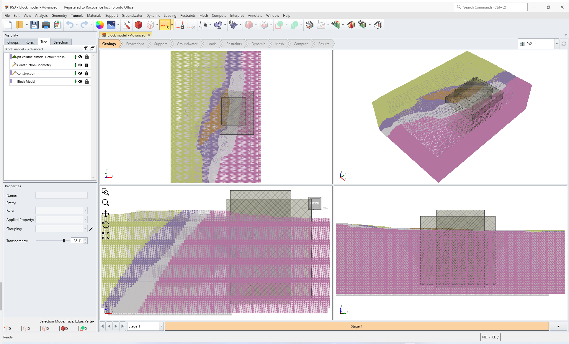
   
4. Browse different child materials in the material dialog and assign the values for stiffness parameters as below:

Rock Types	Material Parameters	Value
AMP	Poisson’s Ratio	0.28
	Young’s Modulus (MPa)	7389.43
HW	Poisson’s Ratio	0.25
	Young’s Modulus (MPa)	12634.4
FW	Poisson’s Ratio	0.18
	Young’s Modulus (MPa)	9493.41
ORE	Poisson’s Ratio	0.23
	Young’s Modulus (MPa)	8601.59
Schist	Poisson’s Ratio	0.3
	Young’s Modulus (MPa)	6143.72

5. Select Strength tab for any of the child materials to check that the selection status of Block Data check boxes should reflect that of Slide3 project with residual strength parameters. Furthermore, RS3 ensures that the block data for peak strength parameters is copied to their corresponding residual pairs.

7.2 Setting up the Plastic Region

1. Under the Visibility Tree, select Construction Geometry.
   
2. Select Materials > Add Plastic Regions. This creates plastic regions which allow element failure within the defined area. For more information on plastic regions, see the Plastic Region Overview help topic.
   

7.3 Apply Hybrid Mesh and Surface Restraints

1. Select the Restraints workflow tab
2. Select Restraints > Auto Restrain (Surface).
   
3. Select the Mesh workflow tab
4. Under the Visibility Tree, select construction.
5. Select Mesh > Define Higher Order Region.
   
6. Select Mesh > Mesh Settings
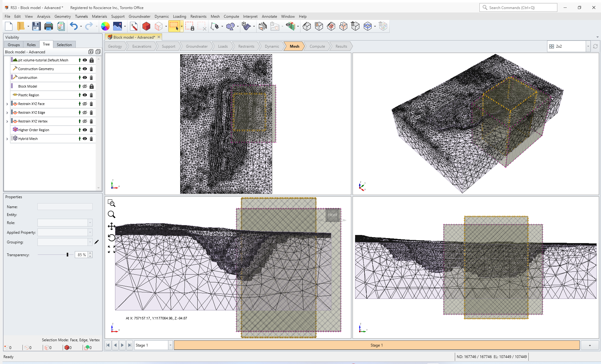
7. Set the Element Type to Mixed 4-Noded and 10-Noded Tetrahedra, and Mesh Gradation to Graded and Select Mesh.
8. Once meshing completes, select OK to close the Mesh Settings dialog. The Model is now ready to conduct SSR analysis.

7.4 Result Comparison

Below shows the 3D Limit Equilibrium slope stability analysis result from Slide3 using Intelligent Search method. The computed failure surfaces with Factor of Safety (FS) of 1.745, 1.749, and 1.750 are displayed in red, blue, and orange color.

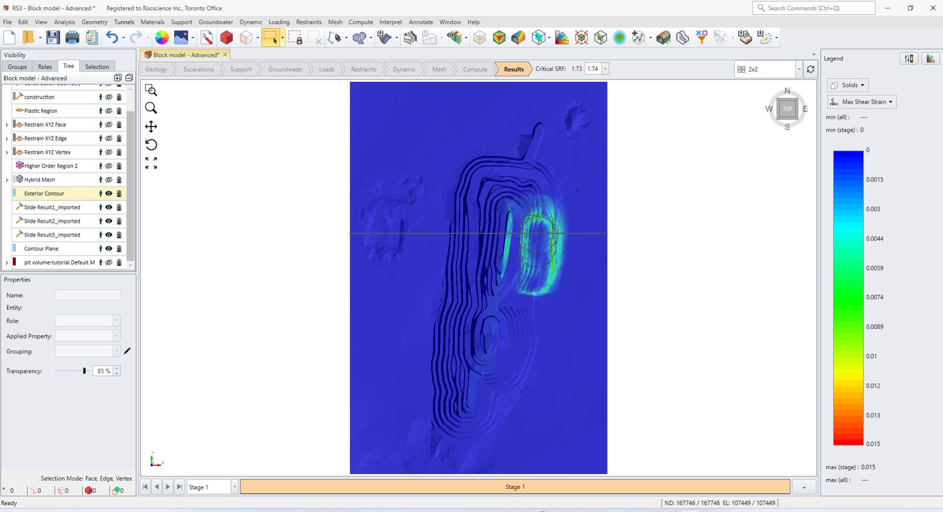
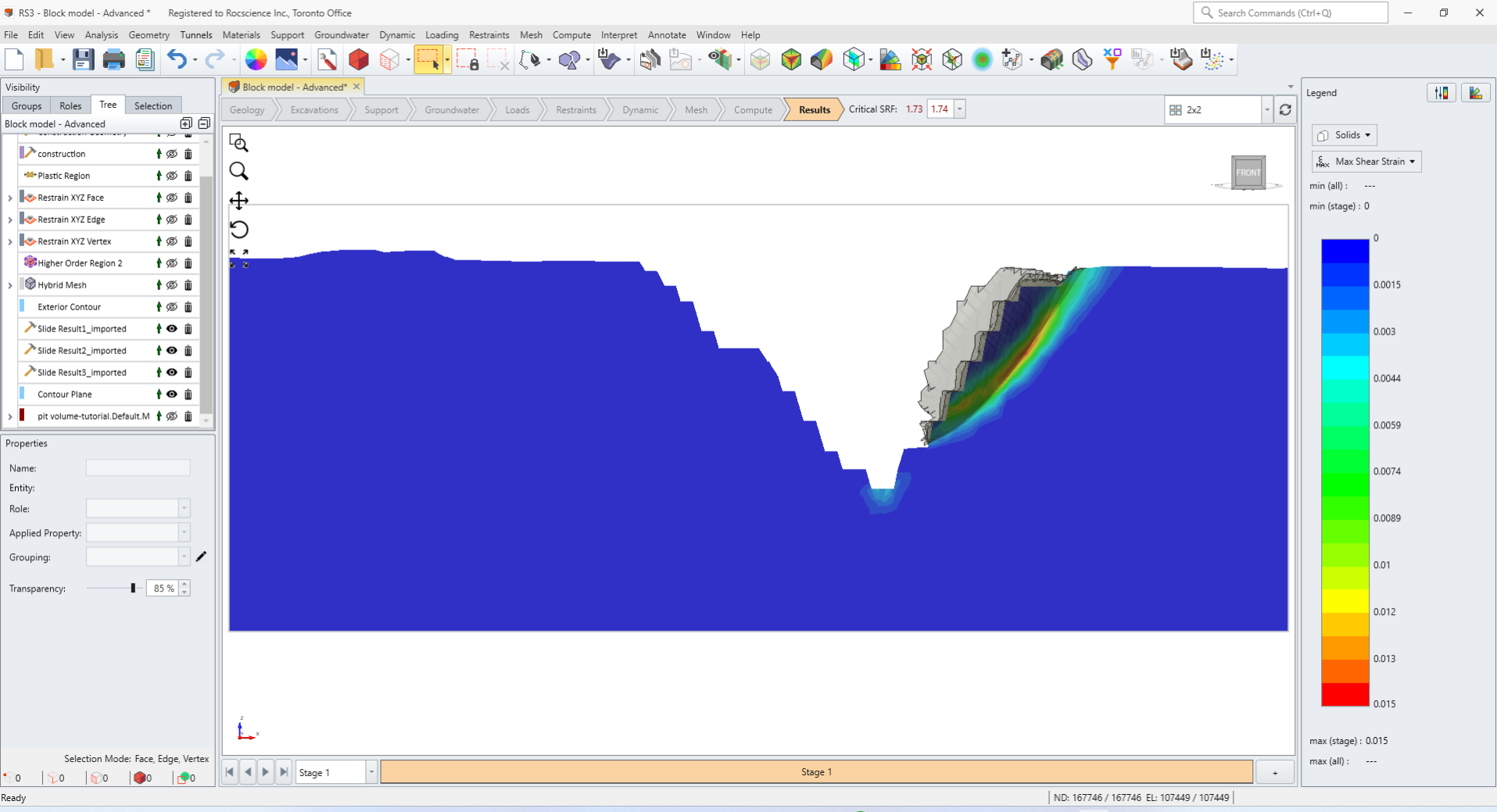
The SSR analysis conducted with RS3 results in the critical SRF of 1.74. Figures below shows maximum shear strain distribution in different views with failure surfaces from Slide3 (Slide3: Interpret > Import/Export Slip Surface > Export Slip Surface and RS3: Interpret > Import Slide3 Results). The maximum extent of shear strain anomaly shows a close correlation with the failure surface of 1.750 FS and the trace of high shear strain can also be traced following the other failure surfaces as well.

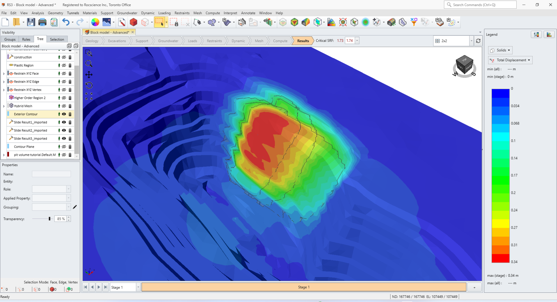
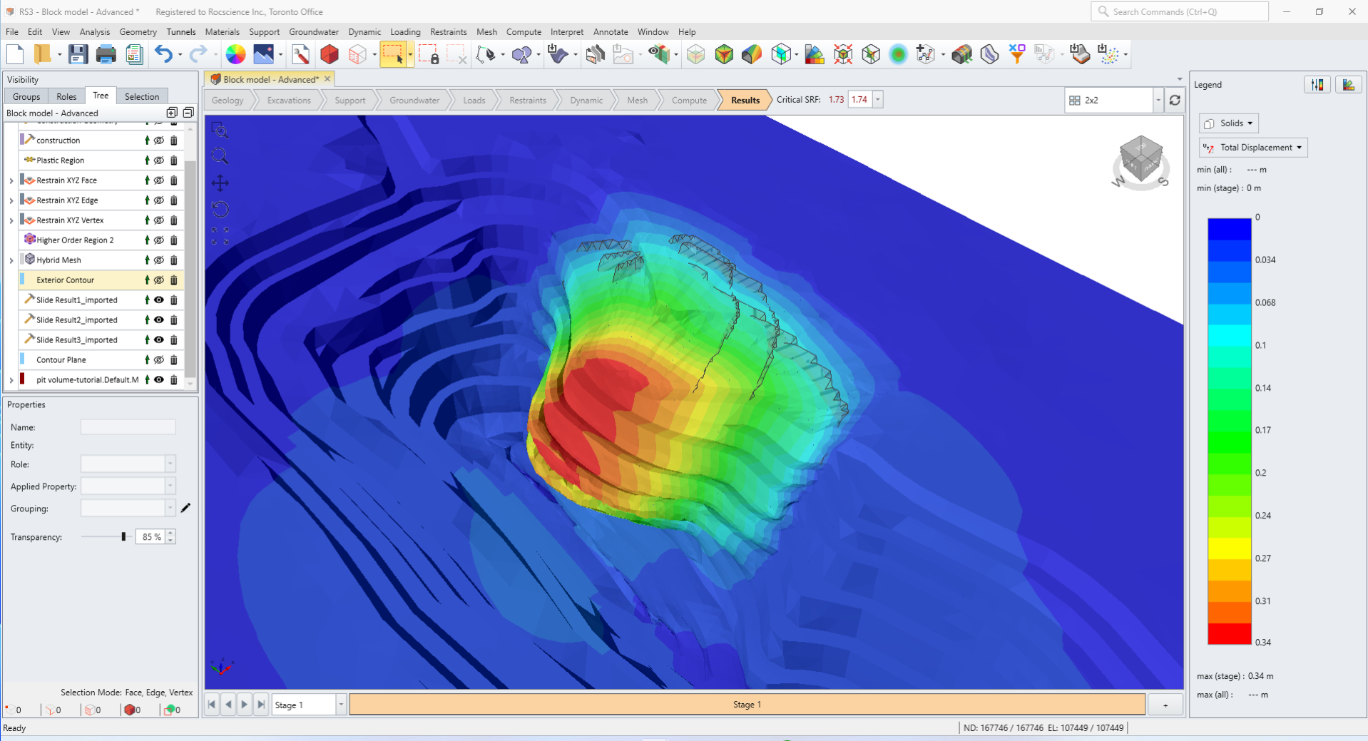
Below shows a closer view of the investigated domain of the pit with maximum displacement contour. Consistent to the observation from maximum shear strain contour, the deformation is highly concentrated in the region of the failure surface of lowest FS and the extent of deformed region is in a close match with the failure surface of 1.750 FS.