Methods

Three-dimensional limit equilibrium slope stability analysis is directly analogous to 2-dimensional methods.

• In 2D a sliding mass is discretized into vertical slices
• In 3D a sliding mass is discretized into vertical columns with a square cross-section

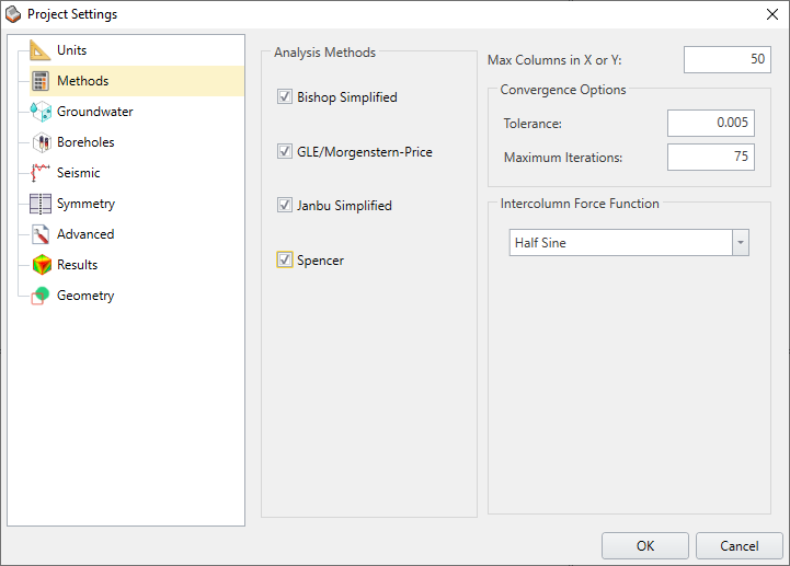
The Methods page in the Project Settings dialog allows you to choose the Analysis Method(s) and Convergence Options.

Analysis Methods

Project Settings > Methods allow users with four analysis methods to choose from as shown in the figure below:

The 2D methods of slices (Bishop, Morgenstern-Price (GLE), Janbu, and Spencer) which are based on satisfying force and/or moment equilibrium, can be extended to a 3D method of columns, where forces and moments are solved in two orthogonal directions. Vertical forces determine the normal and shear force on the base of each column.

The main assumptions for each method are the same in 2D and 3D:

• Bishop - moment equilibrium
• Janbu - force equilibrium
• Spencer - force and moment equilibrium with constant intercolumn force angle
• GLE - force and moment equilibrium with intercolumn force function

For further information see the Slide3 Theory Overview document.

Max Columns in X or Y

The discretization of a sliding mass into vertical columns is based on the following assumptions:

• all columns have a square cross-section of equal area
• columns are aligned with the X-Y axes

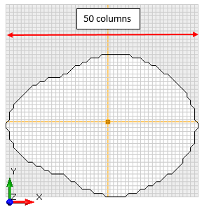
Therefore the sliding mass is always discretized into a grid of square columns with equal cross-sectional area.

Max Columns in X or Y is the maximum number of columns for a sliding mass in either the X-direction or Y-direction (the selected direction is automatically determined by the Slide3 engine and depends on the shape of the slip surface). Since the columns all have a square cross-section with equal area, specifying the number of columns in one direction also determines the total number of columns for a sliding mass. Because of the above assumptions, the total number of columns generated for different slip surfaces is variable.

Convergence Options

The Convergence Options include Tolerance and Maximum Iterations as described below.

Tolerance

The Tolerance is the difference in safety factor, between two successive iterations of the limit equilibrium analysis procedure, at which the solution is considered to have converged, and the iteration process is stopped. The default value of 0.001 is recommended. Much smaller values will increase the computation time, and may lead to convergence problems.

Maximum Iterations

The Maximum Iterations is the maximum number of iterations allowed in the limit equilibrium analysis, for each slip surface. Although the default value is 75, it should be noted that for a typical problem, a much fewer number is required for convergence. If a given slip surface requires more than say, 20 iterations, incorrect material properties, or very low safety factors, may be the cause, and the user should check their model input carefully. If the Maximum Number of Iterations is reached, then the iteration process is terminated for that slip surface, and the last calculated value of safety factor is recorded.

Intercolumn Force Function

The Intercolumn Force Function option is only applicable for the GLE analysis method. The default function is Half Sine. You can also choose Constant for the Intercolumn Force Function. If you select the Change button you can view the shape of a function.

Notes:

• Each analysis method makes assumptions about the angle of the resultant intercolumn forces. For the Bishop and Janbu methods, the angle of the resultant intercolumn forces is horizontal, since both methods assume zero intercolumn shear force.
• For the Spencer method, a constant intercolumn force angle is computed during the analysis.
• For the GLE method, the intercolumn force function determines the angle of the resultant intercolumn forces, across any row of columns in the X or Y directions.

Important note on computing multiple methods:

When computing multiple methods at once (e.g. Spencer, GLE, and Bishop), it's possible that the user may get different results when compared to computing a single method alone (e.g. Spencer only). The reason for this is that at the end of the computation, Slide3 takes all the global minima surfaces from all methods, and computes them with the other methods, in case one turns out to be a better surface.

For example, say at the end of a computation where Spencer, GLE, and Bishop were used, Spencer finds Surface 1 as the global minimum. GLE finds Surface 2. Bishop finds Surface 3.

Subsequently, Surfaces 2 and 3 are recomputed with Spencer. Surfaces 1 and 3 are recomputed with GLE. Surfaces 1 and 2 are recomputed with Bishop.

For Spencer, if Surface 2 gives a lower factor of safety than the original Surface 1, then Surface 2 will be displayed as the global minimum. On the other hand, if the user was computing Spencer alone, Surface 1 would be the global minimum. The same process applies to the other methods.