3 - Combinations Analysis

In Tutorial 02 - Probabilistic Analysis you learned how to perform a Probabilistic analysis. In this tutorial, you will learn how to run a Combinations analysis.

It is inherent in the SWedge analysis when Block Shape = Wedge (the default) that tetrahedral wedges can be formed only by the intersection of two joint orientations with an optional tension crack. For tetrahedral wedges, SWedge does NOT consider more than two joint planes simultaneously in the analysis.

However, if your analysis input data includes more than two possible joint orientations, running a Combinations analysis allows you to analyze all possible combinations of two joints. The joint orientation data can be entered manually or imported from a Dips file using the Combinations Input Data dialog. You can define a single set of orientation data or two sets. If you define two sets, they can have different strength properties, and all possible combinations (using one joint from each set) are analyzed.

Topics covered in this tutorial:

• Project Settings
• Combination Analysis Type
• Importing Joints from Dips
• Limiting Wedge Size
• Barton-Bandis Strength
• Scatter Plot
• Persistence Scaling
• Stereonet
• Bolts

Finished Product:

The finished product of this tutorial can be found in the Tutorial 03 Combination Analysis.swd7 file, located in the Examples > Tutorials folder in your SWedge installation folder.

1.0 Introduction

In this tutorial, we’ll look at the analysis of a dataset containing 356 joint orientations obtained from a Dips data file. With these 356 measurements of joint orientation, we'll look at how to determine all the possible combinations that can be formed by the 356 joints. We'll look at the practical issues in determining the wedge with the minimum Factor of Safety as well as persistence information to get a better idea of the distribution of wedge sizes and Factors of Safety. Finally, we'll determine the bolt force required to guarantee a minimum Factor of Safety for all combinations.

2.0 Creating a New File

1. If you have not already done so, run the SWedge program by double-clicking the SWedge icon in your installation folder or by selecting Programs > Rocscience > SWedge > SWedge in the Windows Start menu.

When the program starts, a default model is automatically created. If you do NOT see a model on your screen:

2. Select: File > New

Whenever a new file is created, the default input data forms valid slope geometry, as shown in the image below.

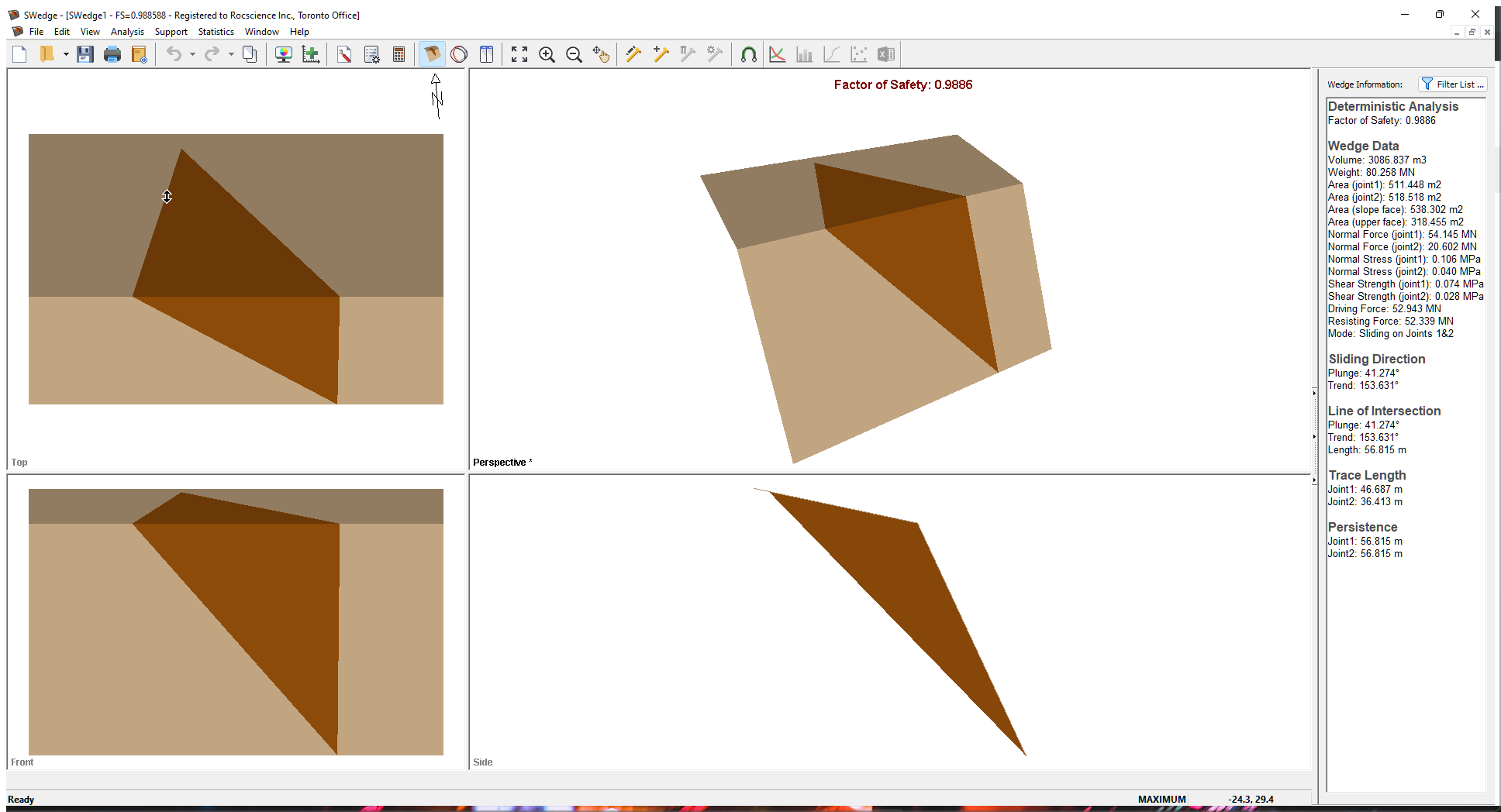
If the SWedge application window is not already maximized, maximize it now so that the full screen is available for viewing the model.

Notice the four-pane, split-screen format of the display, which shows Top, Front, Side and Perspective views of the model. This view is referred to as the Wedge View. The Top, Front and Side views are orthogonal with respect to each other (i.e., viewing angles differ by 90 degrees.)

3.0 Model

3.1 PROJECT SETTINGS

Let's start by specifying a Combinations analysis in the Project Settings dialog.

1. Select: Analysis > Project Settings
2. In theGeneral tab, select Combinations as the Analysis Type.
3. Select Metric, stress as MPa for Units.
4. Press the OK button to close the dialog.

3.2 INPUT DATA

Now let’s define the slope and joint properties in the Input Data dialog.

1. Select: Analysis > Input Data
2. Select the Slope tab and set Dip = 65, Dip Direction = 180, and Height = 20 for the Slope.
3. Set Dip = 0 and Dip Direction = 180 for the Upper Face.
   Since the Dip Direction is the same as for the Slope, you could also check the Use Slope Dip Direction check box.
4. Select the Joints tab.
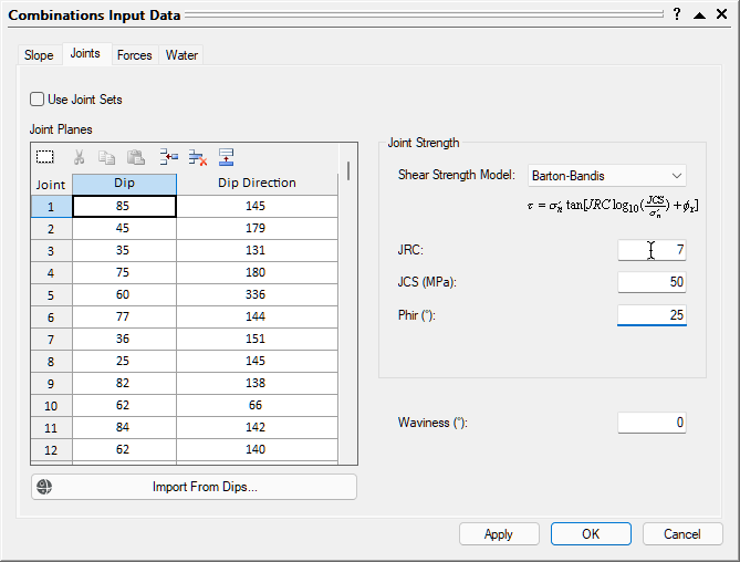
5. Click the Import From Dips button. Go to the Examples > Tutorials folder in your SWedge installation folder and open the Tutorial 03 Combinations.dips8 file.
6. In the Dips Data Import Options dialog, keep the defaults and press the OK button.
   Dips is an industry-standard Rocscience program for plotting joint orientation data on a stereonet. You can also copy and paste orientation data directly from Microsoft Excel or any other spreadsheet program if you do not have Dips. You can also manually define the joint sets by typing the data into the Joint Planes grid in the Joints tab.
7. In the Joints tab under Joint Strength, change the Shear Strength Model to Barton Bandis. Set JRC = 7, JCS [MPa] = 50, and Phir [deg] = 25
8. Click the OK button to save your changes, compute the combinations, and close the Input Data dialog.

4.0 Analysis Results

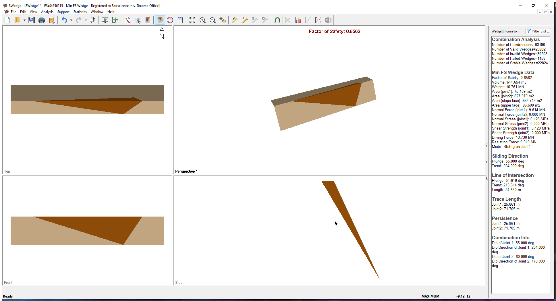
After the analysis is complete, computation of all the possible combinations of the 356 joint planes will occur, as shown in the figure below. Note that the Factor of Safety for the minimum Factor of Safety wedge is 0.6562.

Some other results you should make note of are:

• The results of the Combination analysis are displayed in the Wedge Information Panel in the Sidebar, showing data for the wedge with the minimum Factor of Safety ( Min FS Wedge Data).
• The total Number of Combinations is 63190. The total number of combinations when running one joint set is n(n-1)/2, where n is the total number of joints (356 in this case).
• Since not all combinations produce a wedge, the number of valid combinations is also displayed (Number of Valid Wedges).
• Of these valid wedges, the number of combinations that produce a wedge that is unstable/failed (Factor of Safety < 1.0) and the number of combinations that produce a stable wedge (Factor of Safety >= to 1.0) are also displayed.
• The wedge combination with the minimum Factor of Safety of 0.656 is the wedge formed by joints with Dip/Dip Directions of 55/204 and 60/178. The Weight for this wedge is 16.76 MN.

4.1 SCATTER PLOTS

Now let’s plot the distribution of Factor of Safety vs. Wedge Weight for all the combinations by opening the Scatter Plot Parameters dialog.

1. Select: Statistics > Plot Scatter
2. Make sure the X Axis Dataset is set to Safety Factor and the Y Axis Dataset is set to Wedge Weight.
3. Click OK.

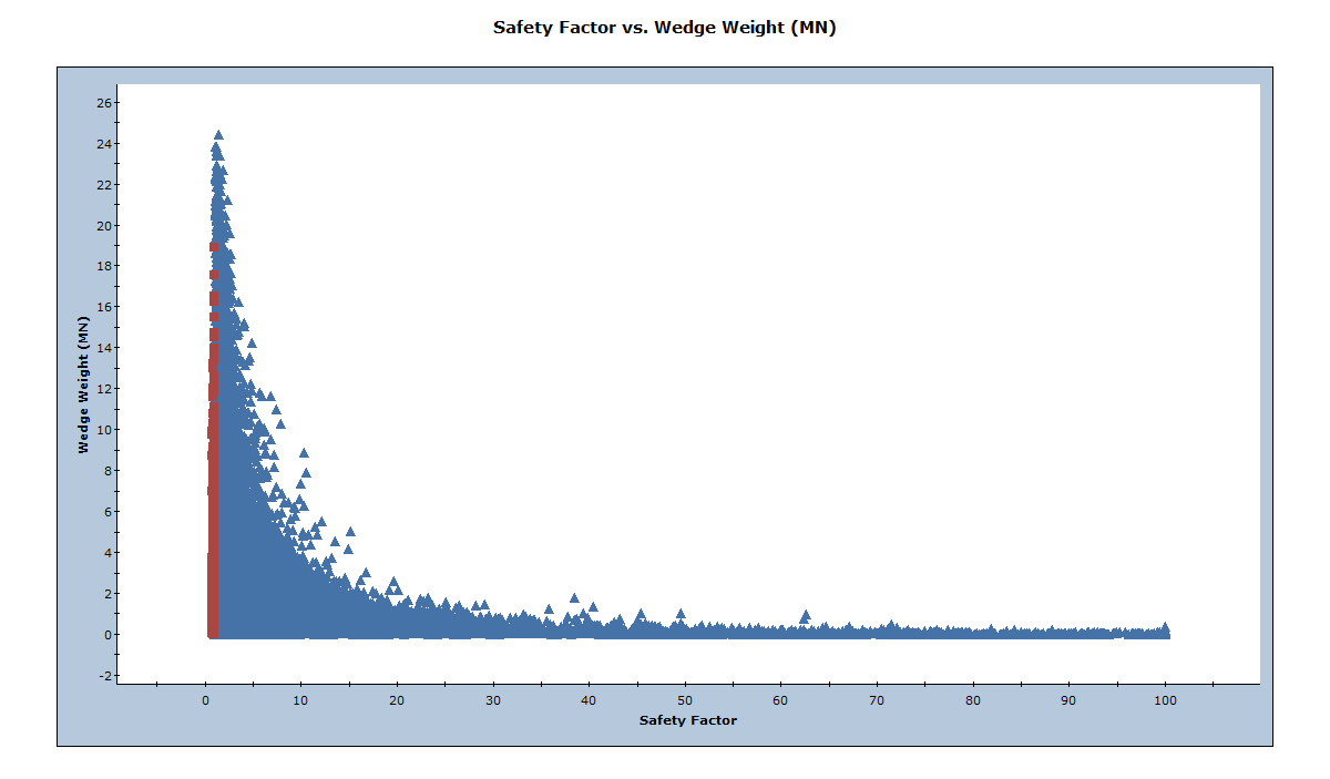
The following figure shows the distribution of Factor of Safety vs. Wedge Weight.

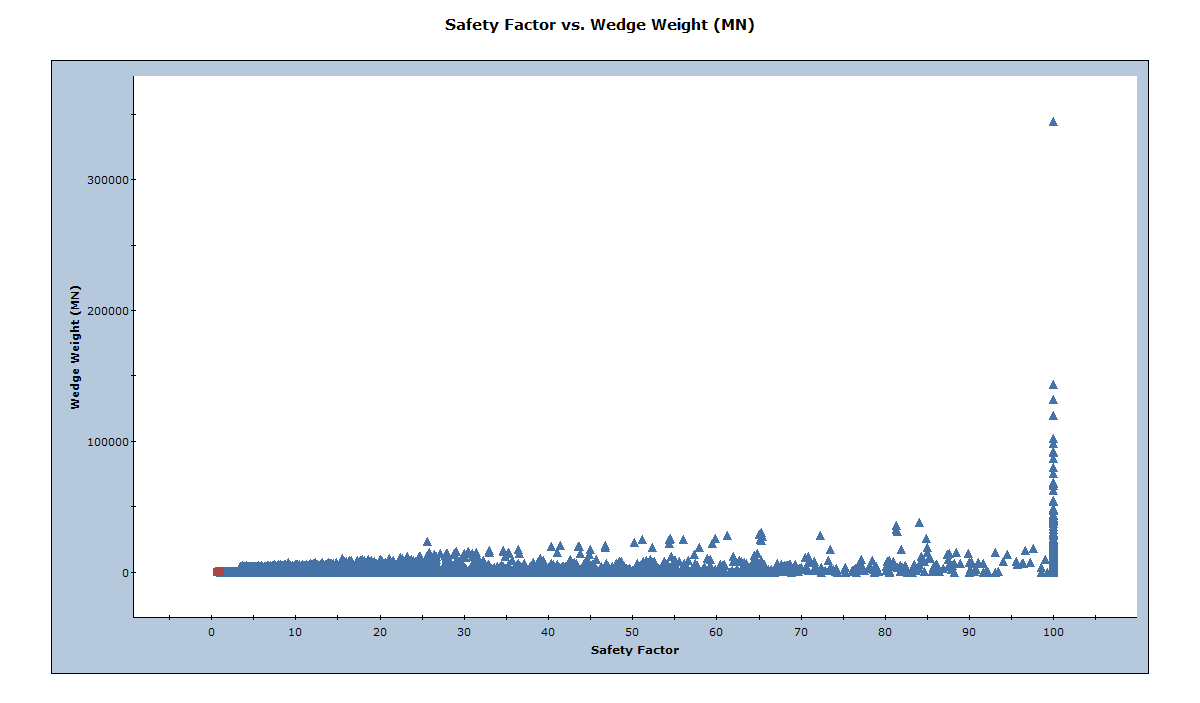
It’s obvious from the above figure that some of the combinations produce huge wedges.

1. To see the wedge corresponding to any of the data points in the graph, double-click the data point in the graph.
2. Double-click the data point furthest in the upper right. This is the point with a Factor of Safety of 100 and a Wedge Weight of around 344000 MN.
3. To switch to the Wedge View, select Wedge View on the Analysis menu or select the Wedge View tab at the bottom of the application window.

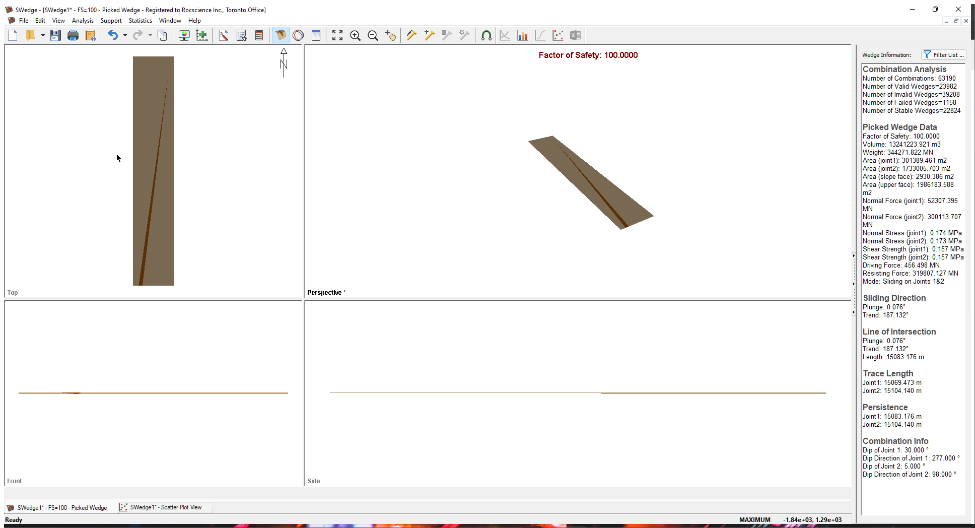
Note the following:

• The wedge with the maximum weight has a persistence and maximum trace length of over 15 kilometers. Clearly, there is no chance a wedge could exist with a joint plane continuity of this magnitude.
• A wedge of this size with a weight of over 344000 MN is clearly not possible so some mechanism should exist for limiting the size of wedges that are formed.

5.0 Limiting Wedge Size

In our analysis we've seen that wedges produced by certain combinations can have an unrealistic size and extension. SWedge therefore provides a number of methods for limiting the size of wedges that are formed in an analysis. To learn about this feature, re-open the Input Data dialog.

1. Select: Analysis > Input Data
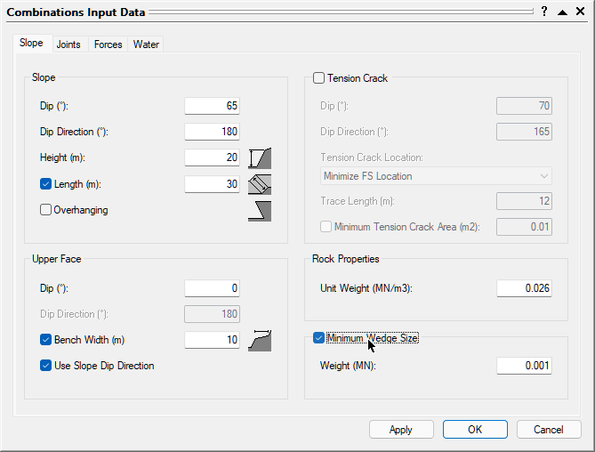
2. In the Slope tab, select the Slope Length (m) check box and enter 30.
   Slope Length is in the same direction as the strike of the slope. Defining Slope Length is just one method of limiting the size of the wedges that are formed.
3. Under Upper Face, select the Bench Width check box and set Width (m) = 10.
   The Bench Width or Upper Face Width is the extent of the upper face measured perpendicular to the slope crest. This distance is measured in the horizontal plane and NOT in the plane of the upper face if it is dipping at an angle greater than 0.
4. Select the Minimum Wedge Size check box and set Weight (MN) = 0.001.
   This option is useful for filtering out very small insignificant sliver-shaped wedges that may be formed.
5. Click the OK button to save your changes, compute the combinations, and close the Input Data dialog.

When the SWedge uses options such as Slope Length and Bench Width to limit the wedge size, wedges that exceed these limits are scaled down so that they fit the slope dimensions. Note that the wedges are NOT removed from the analysis and set as invalid. They are simply re-sized so that they fit the dimensions of the slope. In this way, the program always tries to determine a wedge for a given set of joint orientations.

5.1 ANALYSIS RESULTS

After computation, notice that the Factor of Safety of the minimum Factor of Safety wedge has changed to 0.723, as seen in the figure below.

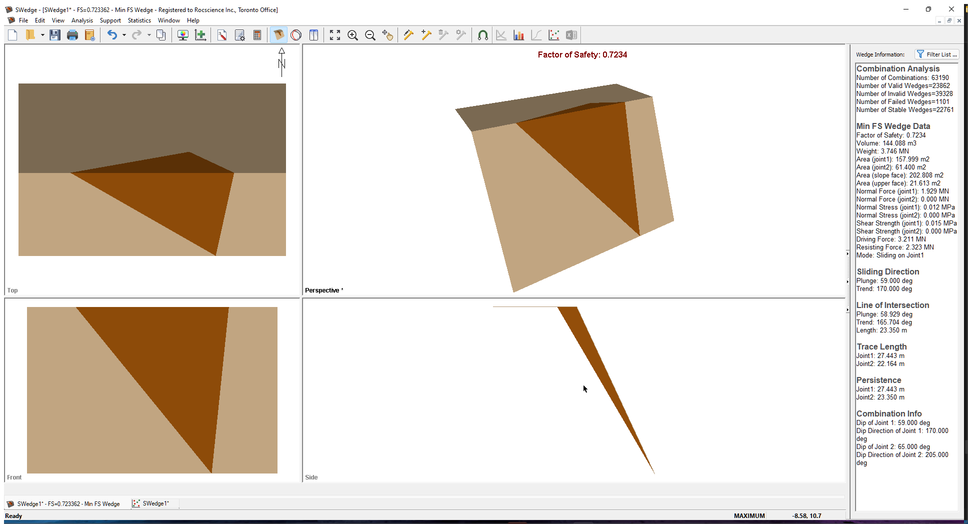
Note the following:

• The minimum Factor of Safety wedge is completely different. If you look at the maximum Trace Length of the unlimited minimum Factor of Safety wedge in the previous section, you’ll see that it exceeds 70m. This is considerably larger than the Slope Length of 30m and Bench Width of 10m used to limit the wedge size. As a result, the unlimited wedge is scaled down in size, which has the effect of lowering its Weight and increasing its Factor of Safety.
• The number of Valid, Invalid, and Failed Wedges has also changed, but not by much. Even with the scaling that exceed the slope dimensions, some wedges cannot be scaled to fit inside the slope.

5.2 SCATTER PLOTS

Now we'll go back to the scatter plot we created earlier in the tutorial.

1. Click the Scatter Plot tab at the bottom of the application window.

Notice that there are no longer the huge wedges that existed in Section 4.1.

6.0 Limiting Wedge Size Using Joint Persistence

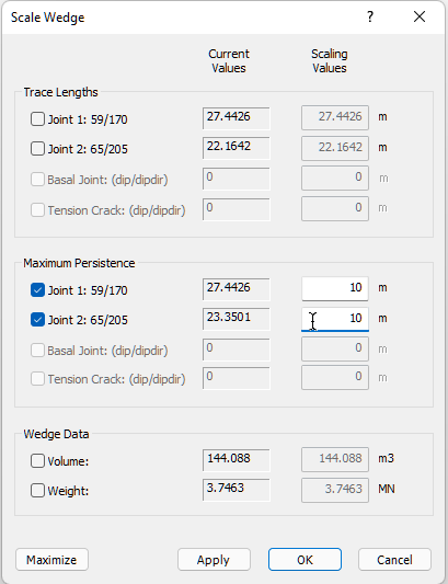
In addition to slope dimensions, you can use joint persistence (the maximum length of a joint in-plane) or trace length information to limit the size of the wedges, using the Scale Wedge dialog.

1. Select Scale Wedge on the Analysis menu.
2. Under Maximum Persistence, select both the Joint 1 and Joint 2 checkboxes and enter Scaling Values of 10 m for both.
3. Press OK to run the analysis and close the Scale Wedge dialog.

6.1 ANALYSIS RESULTS

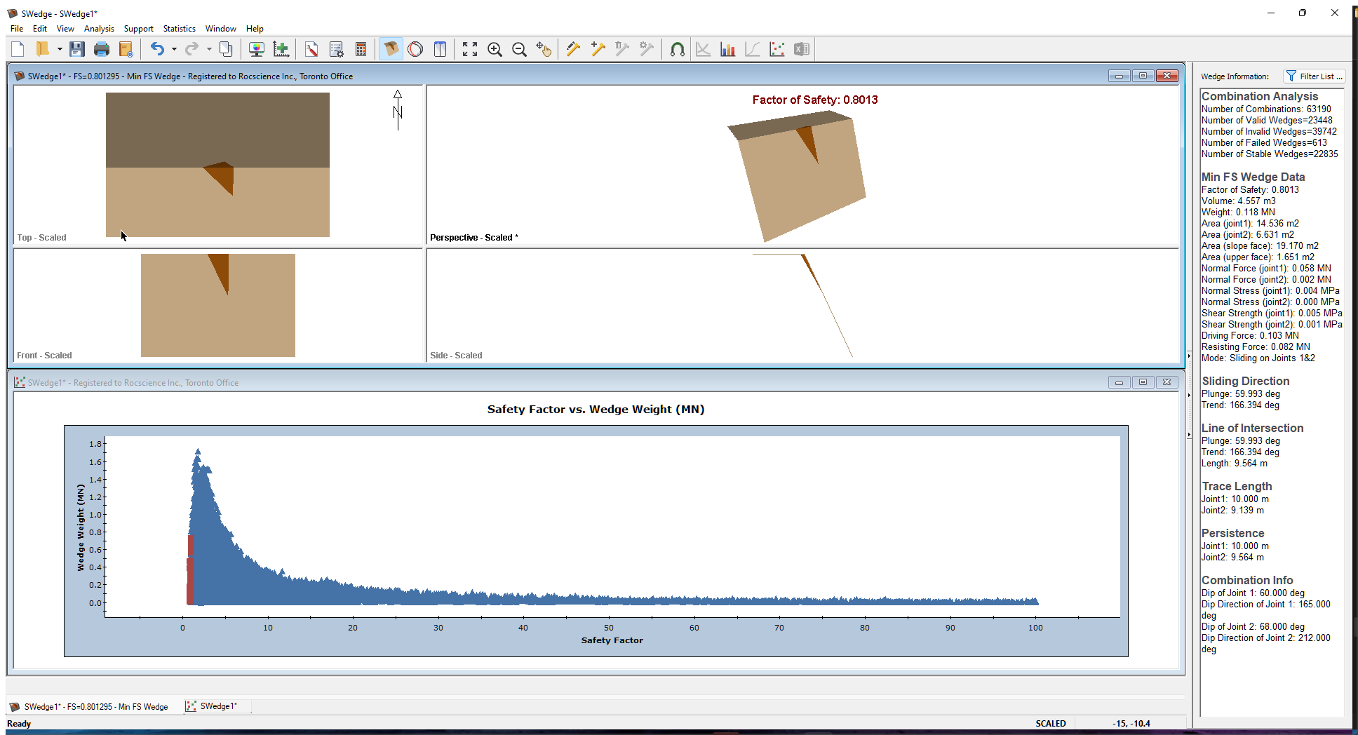
Tile the wedge view and the scatter plot using the Window > Tile Horizontally menu option. Double-click in the Perspective view of the wedge to expand it. Notice that using persistence has the following effect:

• The Factor of Safety has once again increased to 0.801.
• The weight of the wedges has decreased considerably.
• The size of the minimum Factor of Safety wedge is no longer the maximum size wedge that can fit in the slope. It does not extend the full height, length, or width of the slope and has been scaled down to meet the persistence condition.
• The maximum Persistence in the Wedge Information Panel is 10 m, the value you set in the Scale Wedge dialog.

Try double-clicking on a few data points in the scatter plot. Notice that the persistence value for each of these wedges does not exceed the 10 m you defined as the Maximum Persistence in the Scale Wedge dialog.

1. Select View > Show Min FS Wedge again show the wedge with the minimum Factor of Safety.

6.2 PLOT HISTOGRAM

To get an idea of the relative distribution of failed to stable combinations, we can plot a histogram of Factor of Safety again using the Scatter Plot Parameters dialog.

1. Select: Statistics > Plot Histogram
2. Leave theData Type as Safety Factor.
3. Click OK.
   A Safety Factor histogram is displayed.



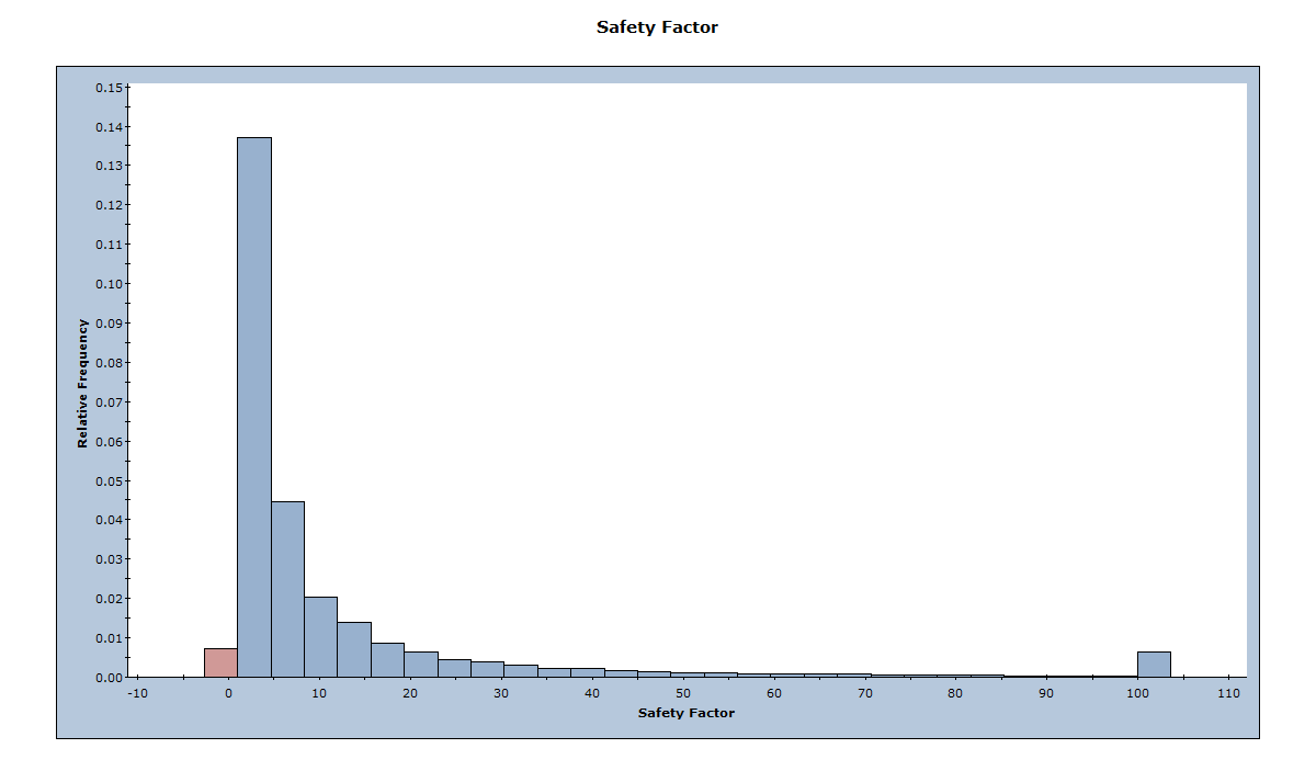
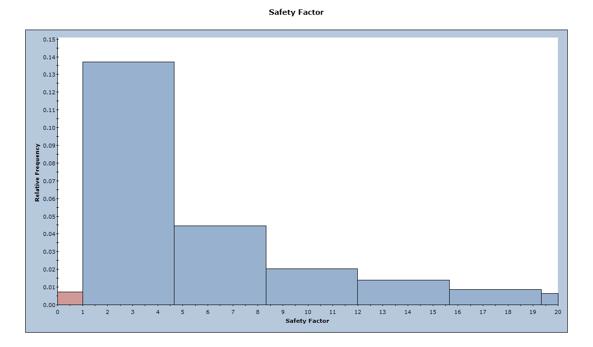
Notice the red bar on the left side of the plot, which represents the unstable wedges with a Factor of Safety less than 1.0. Also notice the bar at the far right side of the plot. This bar represents all the wedges with a Factor of Safety greater than or equal to 100. SWedge truncates the Factor of Safety at 100 so that all wedges with a Factor of Safety greater than 100 are given a Factor of Safety of 100.

Now, lets change the chart properties to look at a distribution of Factor of Safety between 0 and 20.

4. Right-click inside the histogram.
5. In the popup menu, select Chart Properties to open the Chart Properties dialog.



6. In the Axes section, set the Horizontal Minimum to 0 and the Horizontal Maximum to 20. The histogram is updated as you make each change.
   
7. Click Close to close the Chart Properties dialog.

6.3 STEREONET

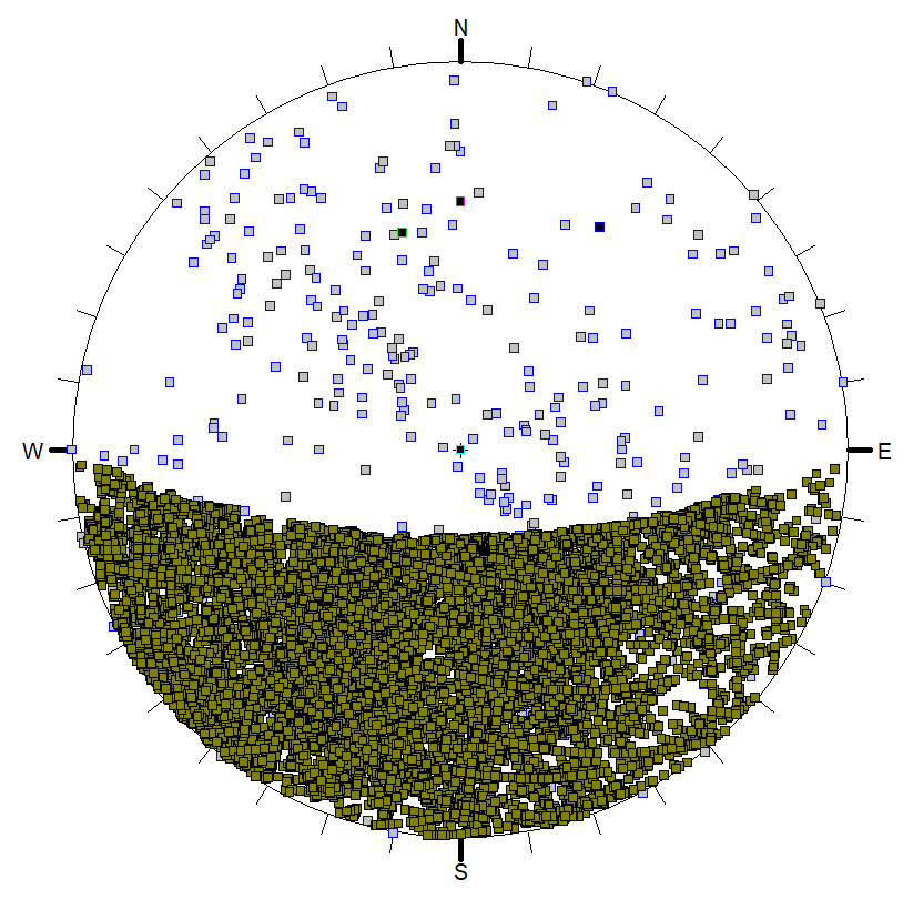
Another tool for visualizing the results of the Combinations analysis is the Stereonet View. In the Stereonet View, you can plot all the poles of the 356 joint planes. You can also plot all the valid lines of intersections (23448 in this tutorial). You also have the option of highlighting the poles and lines of intersection that represent unstable wedges. To open the Stereonet View:

1. Select: Analysis > Stereonet

By default, all the 356 poles are drawn along with the great circles representing the slope, upper face, and the currently set Joint 1 and Joint 2 that are used to plot the 3D wedge view (the minimum Factor of Safety wedge).

Now lets plot the line of intersections and the failed wedges.

2. Right-click in the view and notice that the Show Intersections and Show Planes options are selected in the popup by default.
3. Turn off the Show Planes option by selecting it. These options are also available in the View > Stereonet menu.

7.0 Support

Another aspect of a Combinations analysis is the addition of support to guarantee that all possible wedge combinations will have a Factor of Safety above a certain value. For example, let's look at what bolt force is required to ensure that no wedge has a Factor of Safety less than 1.2. We’ll assume that the bolt is horizontal and trending to the north (directly into the slope face). To do that, let's go back to the Wedge View.

1. Select: Analysis > Wedge View

7.1 BOLT PROPERTIES

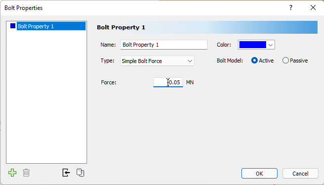
We first need to set up bolt properties using the Bolt Properties dialog.

1. Select: Support > Bolt Properties
2. Select Bolt Property 1.
3. Set Type = Simple Bolt Force.
4. Set Bolt Model = Active.
5. Set Force = 0.05 MN.
6. Click OK.

7.2 ADDING BOLTS

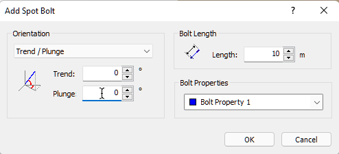
Next, we'll add a bolt using the Add Spot Bolt dialog.

1. Select: Support > Add Spot Bolt
2. Mouse over the Wedge View so the cursor is over the wedge on the slope face.
3. When the cursor changes from to , click the left mouse button to open the Add Spot Bolt dialog.
4. Keep Orientation = Trend / Plunge.
5. Set Plunge = 0.
6. Click OK.

Computation of all the wedge combinations occurs. Each wedge includes a bolt of Bolt Property 1 with a Trend/Plunge of 0/0. After computation, notice that the minimum Factor of Safety wedge has once again changed and that the minimum Factor of Safety is 1.0230.

If we want a Factor of Safety that is no lower than 1.2, we need to increase the bolt Force in the Bolt Properties dialog.

1. Select Support > Bolt Properties to re-open the dialog.
2. Set Force = 0.07 MN.
3. Click OK.
   The Factor of Safety changes to 1.1041.
4. Re-open the dialog and set Force = 0.09 MN.
5. Click OK.
   The Factor of Safety changes to 1.2045.

Note that the changes are linear. We can assume that with Force = 0.09 MN, we can get a minimum Factor of Safety of 1.2.

After computation of all the combinations, the minimum Factor of Safety wedge has a Factor of Safety of 1.2045. Thus a bolt with Force = 0.09 MN and Trend / Plunge = 0/0, ensures that all wedge combinations have a Factor of Safety of at least 1.2. You can verify this by looking at the scatter plot.

Note that you may have to adjust bolt properties a number of times before you reach a point where the minimum Factor of Safety is your design Factor of Safety. This is because different bolt forces can change the minimum Factor of Safety wedge.

This concludes the tutorial.