Surface Altering: Rocscience’s Homegrown Optimization Algorithm
Rocscience researchers published a paper in Georisk journal this month, outlining the optimization algorithm used in Slide2 and Slide3. This algorithm was developed right here in our Toronto office. Read the summary below, or click here to read the full research article.
This article introduces, for the first time, the application of Surface Altering Optimization (SAO) on slope stability analysis using Limit Equilibrium Method (LEM). The study starts by outlining the details of the algorithm and then goes on to put the algorithm to the test with several examples, three of which are presented here:
- How does it compare to Shear Strength Reduction (SSR)?
- How does it compare to no optimization or Monte Carlo Optimization (MCO)?
- How does it fare in a complicated case study with spatial variability?
What is Surface Altering Optimization?
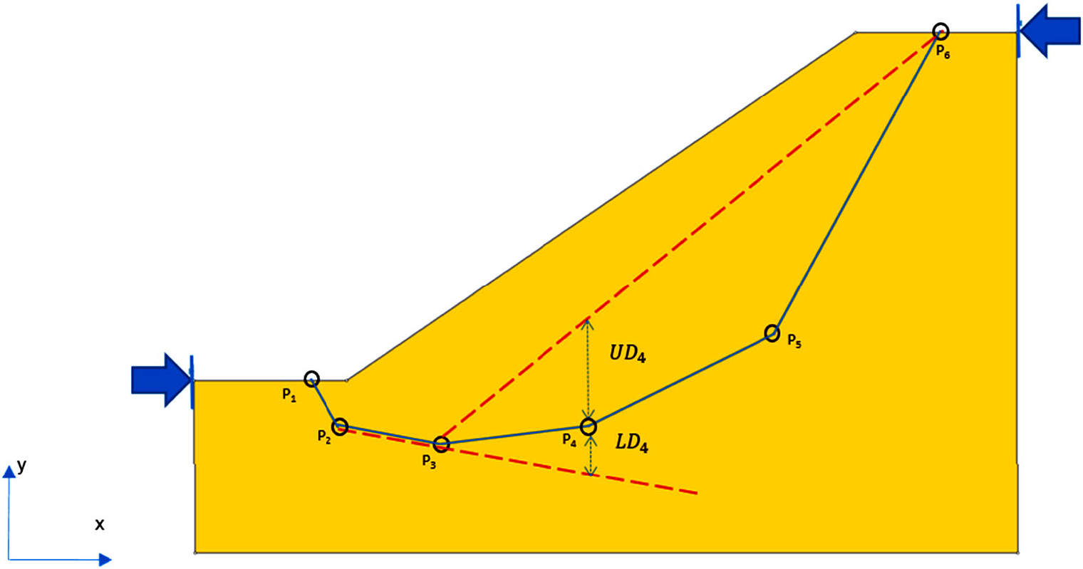
SAO is a technique used to minimize the factor of safety (FS) for a given slip surface by modifying its geometry iteratively. As a local optimization algorithm, it works best when combined with a global search method to calculate the factor of safety. In this way, the computational efficiency of a local optimization algorithm is taken advantage of in the global search. The detailed steps of the algorithm can be found in the paper.
Example 1: How does it compare to SSR?
This first example is taken from literature: Liu, Shao, and Li (2015) compared the results of SSR and LEM approaches for different case examples. The case presented is a multi-layer slope with a thin, weak layer, shown in orange in Figure 2. The challenge for SAO will be whether it can locate the weak layer.
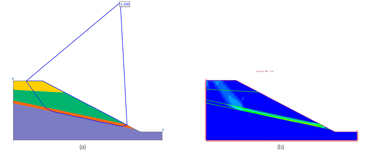
The results of the two analyses are shown in Figure 2. The LEM analysis was computed with a Cuckoo global search and SAO. It can be seen in the results that the failure surfaces themselves are very similar in both the LEM and SSR cases. Furthermore, the FS found by the LEM was 1.10 while the shear reduction factor (SRF) found by the SSR analysis was 1.14. The results are in very good agreement.
Example 2: How does it compare to no optimization or MCO?
When running a LEM analysis in Slide2, the user has the option of running only the global search method (e.g. Cuckoo, Particle Swarm, etc.), or the global search method along with an additional local optimization (either MCO or SAO). This example explores the differences between these three scenarios. An SSR analysis was also computed as additional verification.
The Mount Polley tailings dam was selected to provide baseline geometry and soil properties for this example (Province of British Columbia 2015). The results of the three cases described, as well as of SSR are shown in Figure 3.
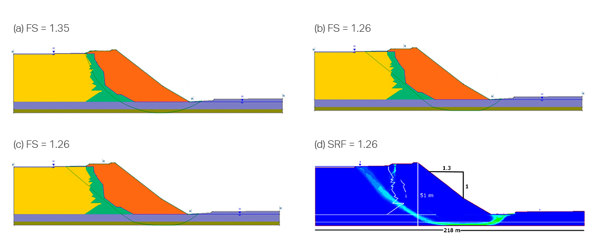
It is immediately apparent that the first case, which does not utilize any additional optimization, gave the worst results, both in FS value and in failure shape. The MCO and SAO cases meanwhile are in very good agreement with SSR.
While the MCO and SAO cases were both shown to give good results, the SAO case did so in a fraction of the time: 20% of the time! This difference in computation time is one of the primary advantages of SAO over MCO.
Example 3: How does it fare in a complicated case study with spatial variability?
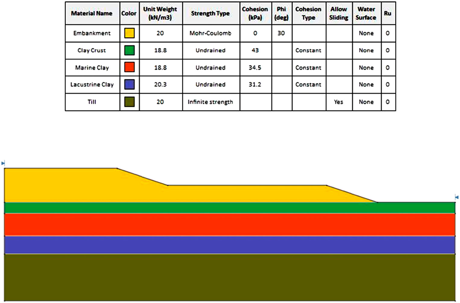
The James Bay dyke presented by El-Ramly, Morgenstern, and Cruden (2002), shown in Figure 4, was selected to provide the baseline geometry and soil properties for this example.
As an extra challenge, spatial variability is considered in this example. Spatial variability describes the consideration of heterogeneity within material sections in Slide2 through the use of random field theory. The analysis method that considers spatial variability in a LEM setting, is called Random Limit Equilibrium Method (RLEM).
The reason why spatial variability is the ultimate challenge for the algorithm, is that the material strength of the slope is now continuously changing, instead of containing stretches of constant strength as before. Hence the algorithm must be fine enough to detect these changes and find the weakest path through the slope.
Two example simulations from the RLEM analysis are shown in Figure 5, along with their respective SSR computations. The SSR computations were done by exporting the random fields in Slide2 as discrete fields and importing them into RS2.
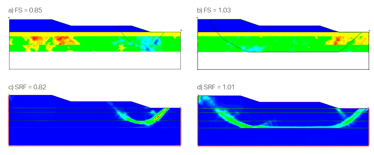
It is evident in this figure that once again SAO was in very good agreement with SSR, even in this complicated case study with spatially varying materials.
Conclusions
This study provides an introduction to the SAO technique in slope stability analysis using LEM. Through the examples above, and countless others, SAO has been found to be a fast and accurate method of optimizing non-circular slip surfaces under the most complex of circumstances.
Reference
Ramin Mafi, Sina Javankhoshdel, Brigid Cami, Reza Jamshidi Chenari & Amir H. Gandomi (2020): Surface altering optimization in slope stability analysis with non-circular failure for random limit equilibrium method, Georisk: Assessment and Management of Risk for Engineered Systems and Geohazards, https://doi.org/10.1080/17499518.2020.1771739.
