31 - Hydraulic Statistics
This tutorial demonstrates the Hydraulic Statistics option in Slide2. Before proceeding with the tutorial, it is helpful to complete Tutorial 5 – Transient Groundwater Analysis, Tutorial 8 – Probabilistic Analysis, and Tutorial 10 – Spatial Variability to familiarize yourself with Groundwater Analysis and the Statistics features used in this tutorial.
Topics Covered in this Tutorial:
- Seepage Analysis
- Hydraulic Statistics
- Probabilistic Analysis
- Spatial Variability
Finished Product:
The finished product of this tutorial can be found in the Tutorial 31 Hydraulic Statistics.slmd data file. All tutorial files installed with Slide2 can be accessed by selecting File > Recent Folders > Tutorials Folder from the Slide2 main menu.
1.0 Introduction
Similar to the principles behind statistical analysis of soil strength properties and determining probability of failure (PF), the Hydraulic Statistics feature allows you to vary hydraulic properties of a material randomly or spatially which accounts for uncertainties in the material parameters. The effects of altering these parameters are most apparent in pore pressures which has a significant effect on the failure surface. For example, if saturated permeability Ks is randomly defined, the speed that water flows through a soil profile can drastically vary and lead to different results between transient stages.
Hydraulic Statistics allows you to:
- Randomly define hydraulic properties of materials
- Cross-Correlate between two hydraulic properties of the same or other material
- Define Spatially variable hydraulic properties
- View final pore pressure results of each individual sample
- View specific hydraulic data from defined query points.
Refer to the Hydraulic Statistics topic for more details.
2.0 Model (Default)
- Select File > Recent Folders > Tutorials Folders to open the Slide2 tutorials folder.
- Select Tutorial 31 Hydraulic Statistics – starting file.slmd and click Open.
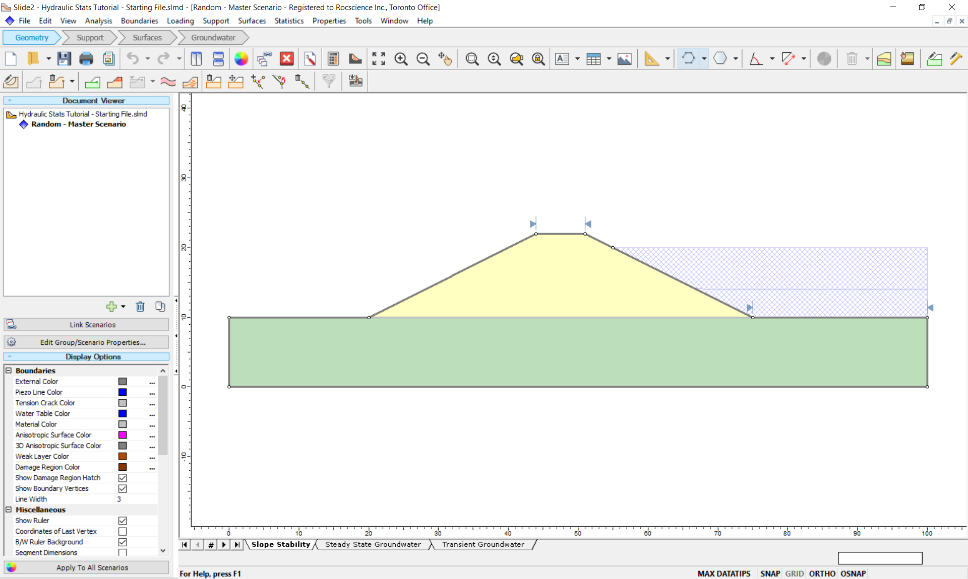
In the first scenario called “Random,” the model consists of two pre-defined materials. The model uses a non-circular PSO analysis using Spencer’s method.
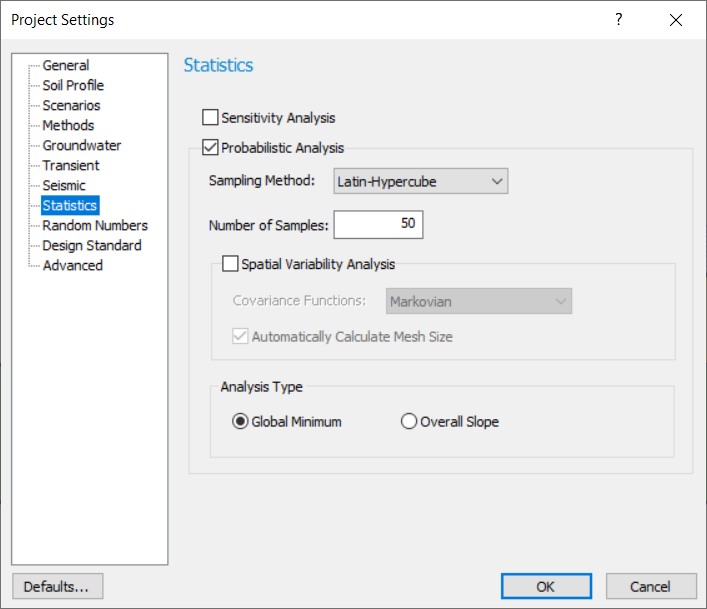
- Go to Analysis > Project Settings
 and select the Groundwater tab.
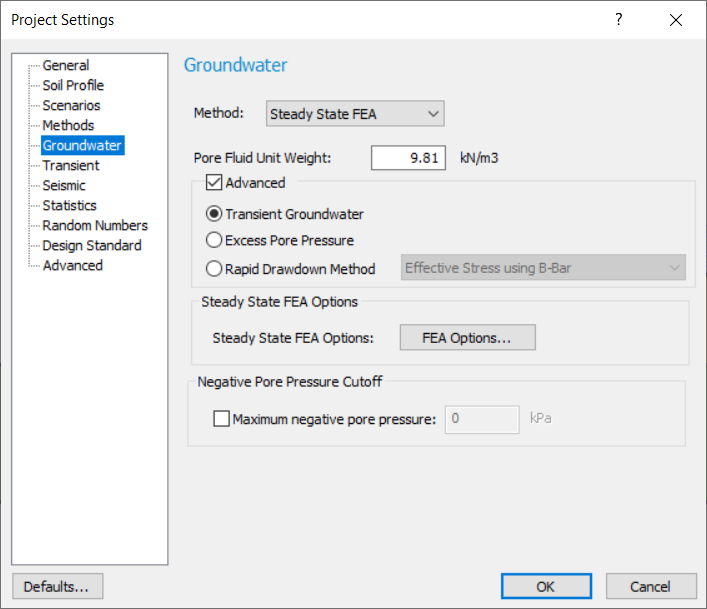
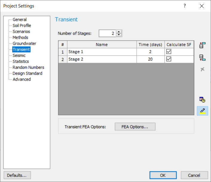
Note that the model is using Steady State FEA analysis as its initial condition groundwater method with transient analysis. Moving to the Transient tab shows that there are two stages defined.
2.1 Hydraulic Properties
When FEA is used (Steady State FEA groundwater and/or transient analysis), each material will have defined groundwater parameters.
- Select the Groundwater workflow tab

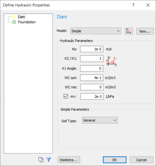
- Select Properties > Define Hydraulic Properties in the menu or click on the Define Hydraulic Properties
 icon.
icon. - For each of the two materials ensure that they have the following defined Saturated Permeability Ks:
| Material | Dam | Foundation |
| Model | Simple | |
| Ks (m/s) | 1e-05 | 1e-08 |
| Soil Type | General | |
2.2 Hydraulic Statistics tab – Random Variables
Now we can define which parameters we want to statistically vary.
- Select the Groundwater workflow tab, select Statistics > Hydraulic
 from the menu, and then select the Dam material.
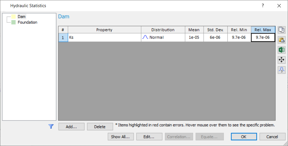
 - Like material statistics, click the Add button and select Ks to be defined as Random.
- Ensure the variable is using Normal Distribution and click Finish.
- Ensure the following Random Variables are defined using the statistical parameters in the table below.
- Repeat the following for the Foundation material with the respective parameters and click OK when finished.
| Property | Mean | Std. Dev. | Rel. Min. | Rel. Max |
| Ks – Dam | 1e-05 | 6e-06 | 9.7e-06 | 9.7e-06 |
| Ks – Foundation | 1e-08 | 1.2e-08 | 9e-09 | 9e-09 |
3.0 Hydraulic Spatial Variability
The hydraulic statistics feature also allows you to spatially define hydraulic properties. To save time, we’ll create another model so both can be computed at the same time.
- Save your project, and duplicate the existing “Random” scenario and rename it as “Spatial.”
- Select Analysis > Project Settings, select the Statistics tab and tick the checkbox beside Spatial Variability Analysis.
- Untick Automatically Calculate Mesh Size. Click OK to close the dialog.
- Go to the Groundwater workflow tab and select Statistics > Hydraulic
 to open the Hydraulic Statistics Dialog.
 - Select the Dam material and tick the checkbox beside the Spatially Variable Material.
- Enter a Correlation Length of 15m for both the X and Y directions, and set the Mesh size to 3.
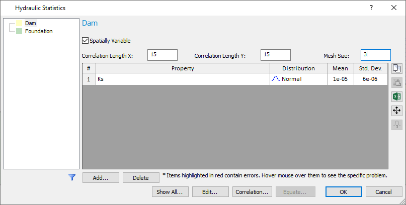
- Repeat for the Foundation material. Click OK to close the dialog.
3.1 Property Viewer – Modeler
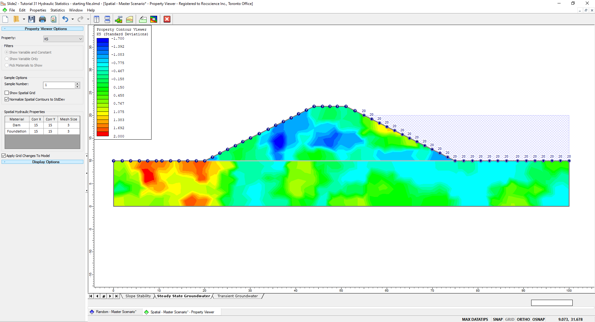
We can preview the generated spatial fields similar to strength parameters using the Property Viewer.
- Select Analysis > Property Viewer

- Set the Property to KS.
- Tick the Normalize Spatial Contours to StdDev in the Property Viewer Options.
- Use the arrows beside Sample Number to view the different spatial fields for the current property
4.0 Hydraulic Query
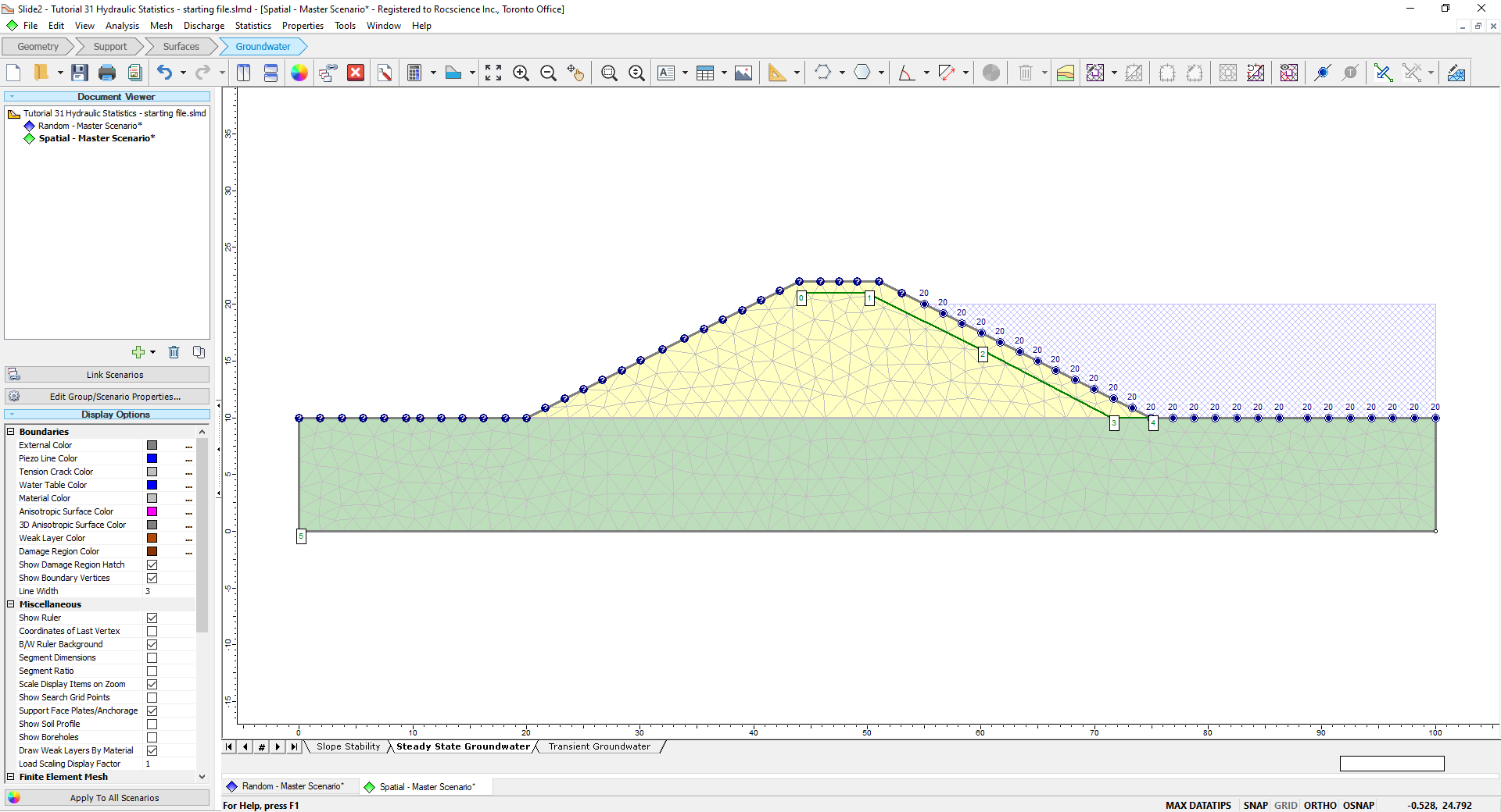
We can view specific hydraulic data for a set of points using the Hydraulic Query feature.
- In the Spatial scenario, select Properties > Hydraulic Query

- While you can select any location, we’ll input the points specifically using the table option. Enter ‘t’ and press the ENTER key.
- Enter the following coordinates in the table as shown below:
- Click OK to close the dialog. Press ENTER once the query appears on the model.
| X | Y |
| 44 | 21 |
| 50 | 21 |
| 60 | 16 |
| 71.5 | 10 |
| 75 | 10 |
5.0 Compute and Interpret
Now that the hydraulic parameters have been randomly defined, we can compute and view results.
- Select the Geometry workflow tab and then select Analysis > Compute
 . Notice during computation for one scenario there will be two groundwater computations, the first for deterministic, and the second for probabilistic.
 - When computations are done, select Analysis > Interpret
 to view the results. This will launch the Interpreter.
 - Ensure you’re viewing Stage 1 for both scenarios. Select the Tile Windows
 button (or select Window > Tile Vertically) to view both the random and spatial results.
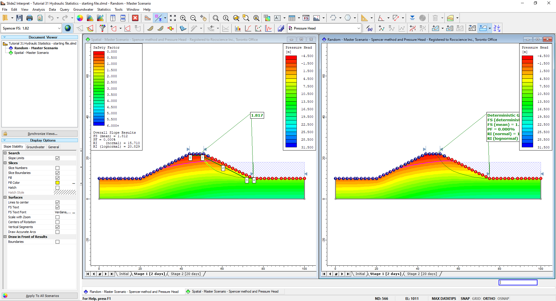
Like statistical analysis for strength parameters, we can see the same statistic results such as the probability of failure, scatter plots, histograms, etc. We can view the scatter plots of Ks versus Spencer FS.
- Ensure the Random scenario result is selected and select Statistics > Scatter Plot

- Ensure the Horizontal Axis
is Dam: Ks (m/s) and the Vertical Axis is Factor of Safety – Spencer.
- Click Plot to create the scatter plot.
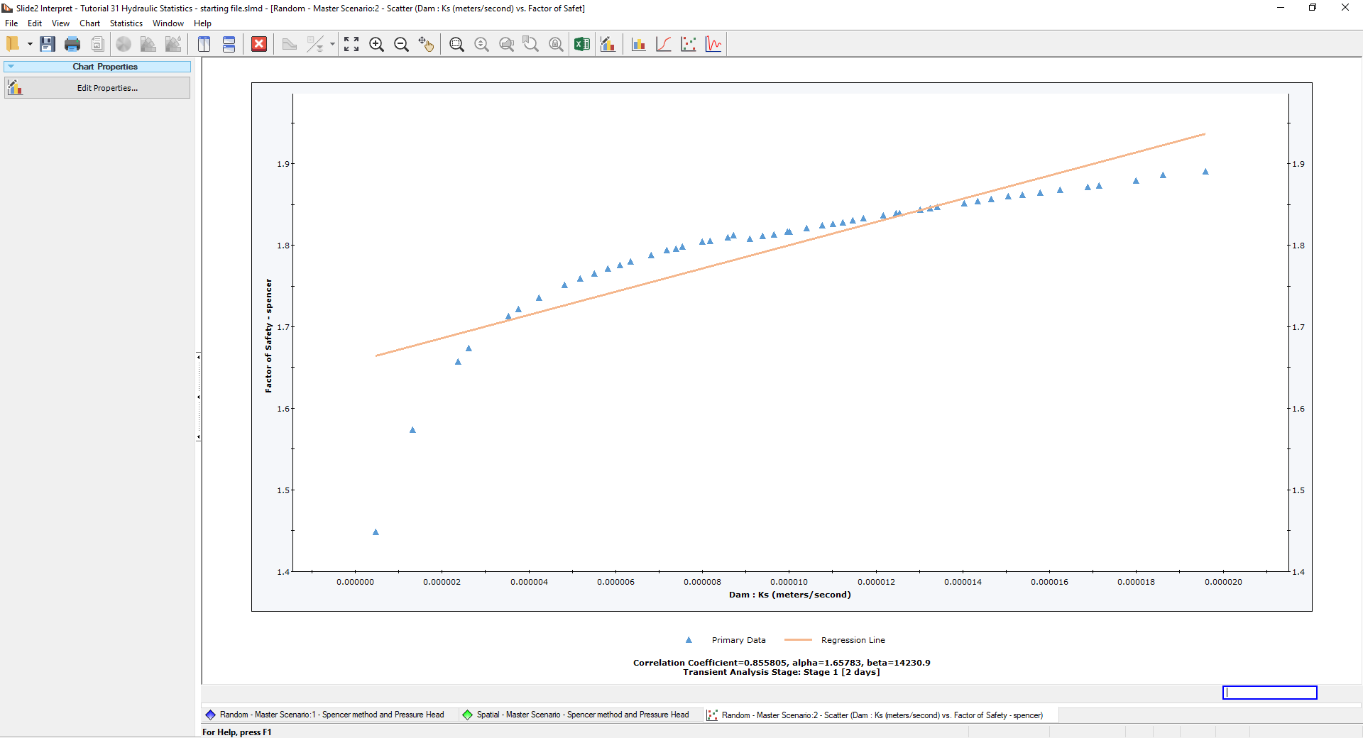
We see that as the permeability increases for the dam, the resulting factor of safety is increasing. Repeating the previous steps for the Foundation material, we also see following scatter plot:
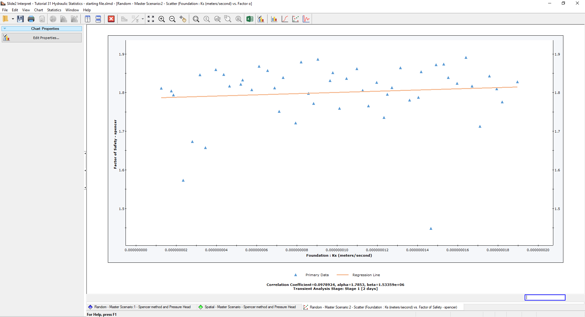
It may be the case that because the surface is failing through the dam, the overall effect of permeability in the foundation would not have any distinct correlation with the factor of safety.
5.1 Property Viewer – Interpreter
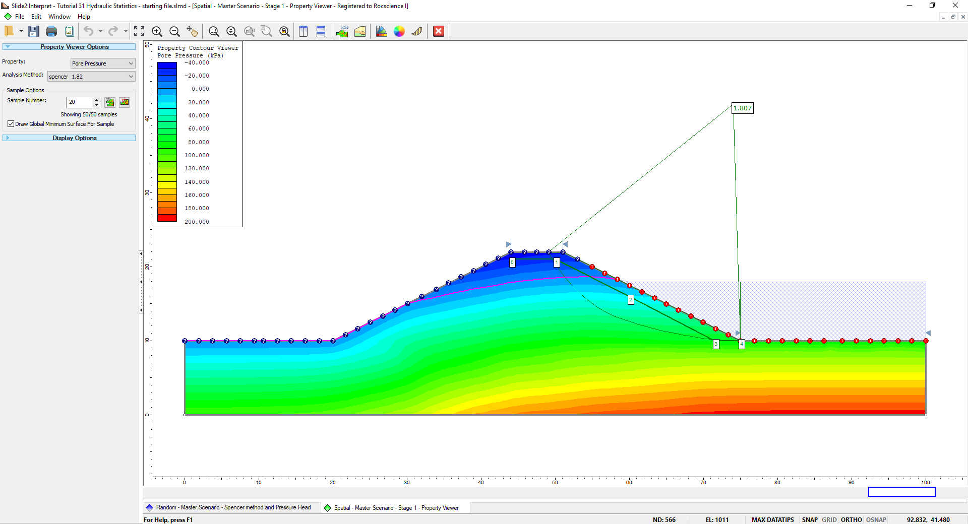
In addition to the same spatial field viewer functionality in modeler, we can view each of the pore pressure results for each sample for each stage using the Property Viewer.
- Ensure the current view is Stage 1 in the Spatial scenario.
- Open the property viewer by selecting Analysis > Property Viewer
 (or click on the icon in the toolbar).
 - On the left side, set the Property to Pore Pressure.
- Using arrows next to Sample Number, flip to sample 20 and view the pore pressure data.
- Switch the property to KS and tick the Normalize Spatial Contours to StdDev checkbox as before.
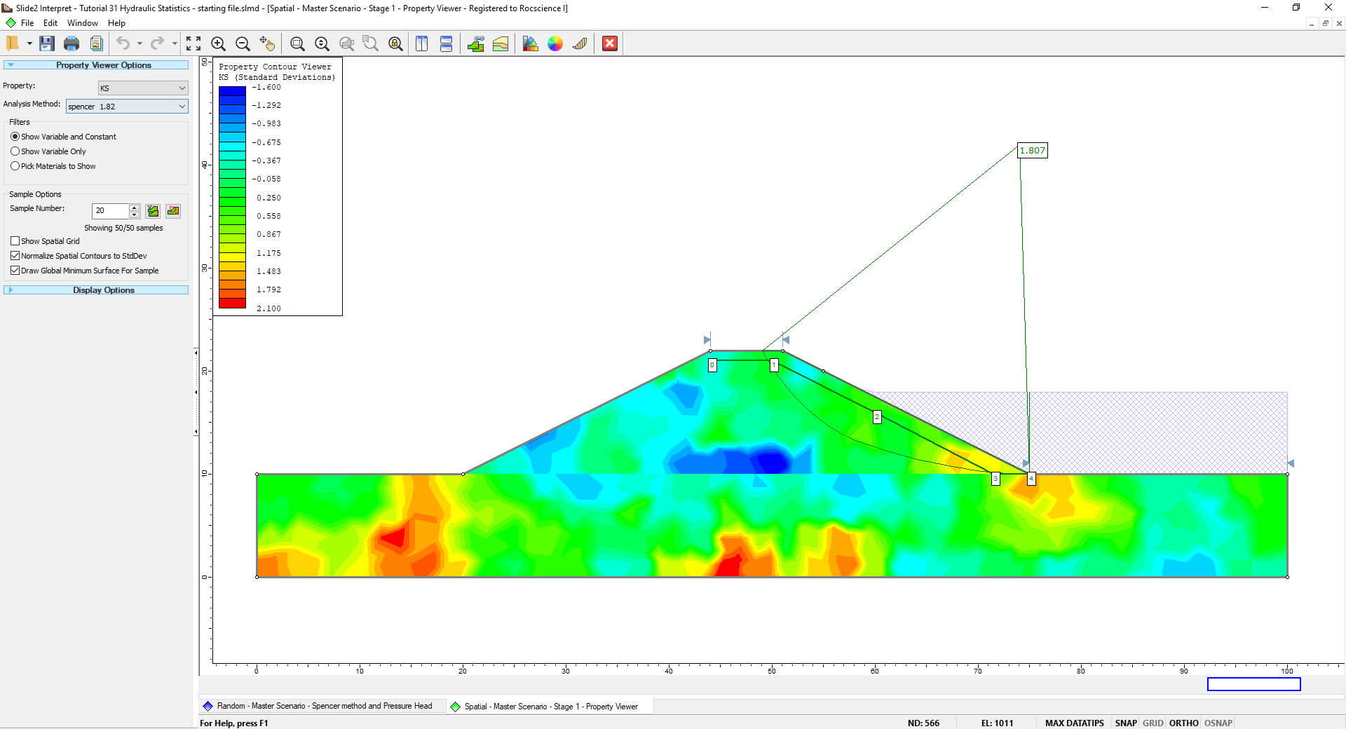
Depending on the spatial distribution of permeability, the pore pressures can be noticeably different between samples. This can also be seen when comparing the phreatic surfaces between samples. Notice the phreatic surface of the following sample is different compared to the previous sample.

5.2 Hydraulic Query Data View
With the addition of the query in the analysis, the data recorded for each of the query points can now be viewed using the existing statistical features.
- Close the property viewer, and in the Spatial scenario, select Statistics > Scatter Plot
 .
. - Change the Horizontal Axis to Total Discharge Velocity and the Vertical Axis to Pore Pressure.
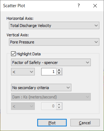
- Click Plot and untick all the query points except for query points 3 and 4.
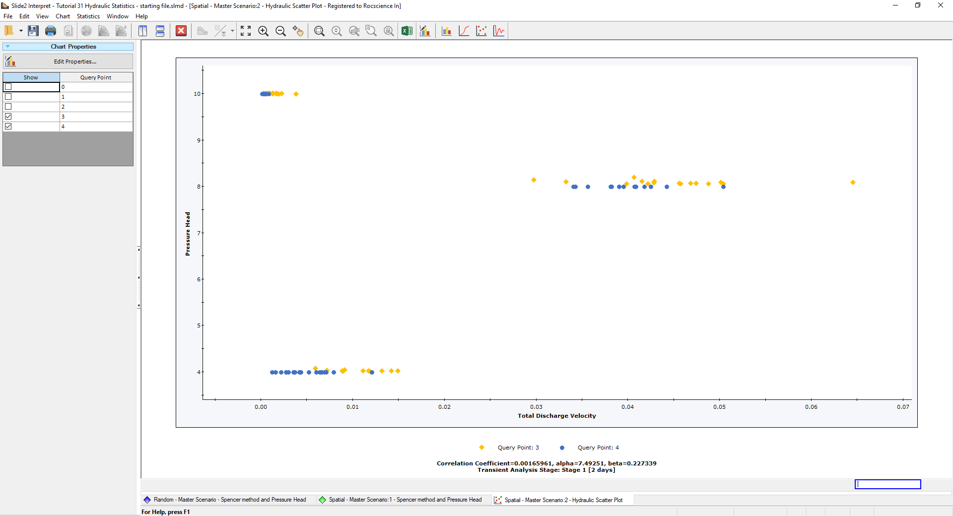
Data can be viewed per query point for all samples or in the aggregate by toggling the query points on or off in the left pane under chart properties. In this case, we see the data varies drastically between the two query points, with one closer to the top of the slope and one near the toe.
6.0 Additional Exercise
Sensitivity Analysis is available to use for hydraulic properties. Note however that only the factors of safety will be visible on the Sensitivity Plot as with all other sensitivity analyses results. No unique pore pressures and/or query results are available for Sensitivity Analysis.
Cross Correlation between hydraulic properties is also available as a feature for hydraulic stats, similar to material stats. Consider defining correlation between the model materials as an additional exercise.
Statistical analysis with soil strength properties can be done simultaneously with Hydraulic Statistics. Consider defining soil parameters as random and/or spatial to see their effects in conjunction with Hydraulic Statistics as an additional exercise.
Depending on the model, computation times could be drastically increased. It is recommended to utilize the Response Surface sampling method to drastically decrease the required amount of computation. This can be set in Analysis > Project Settings and changing the sampling method to Response Surface.
7.0 Summary
This tutorial demonstrated the different usages and features of the Hydraulic Statistics feature to randomly and spatially define hydraulic properties. Using the process shown here, analyses can now account for inherent variability in hydraulic properties and can be analyzed using tools such as the property viewer and the Hydraulic Statistics Query. The Hydraulic Statistics feature is a powerful tool to enhance your probabilistic analysis.
